Automation of soil-structure interaction finite element modelling using Python coding and the project BIM model

Introduction

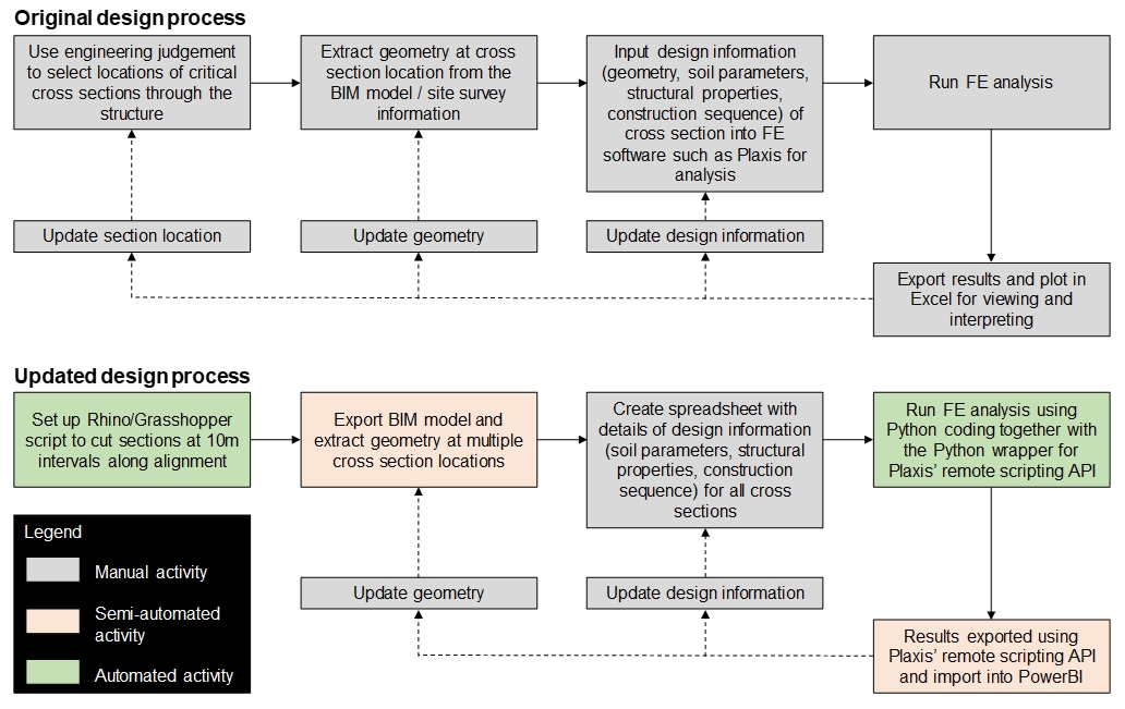
The design of underground structures using 2D geotechnical finite element (FE) modelling typically involves the selection of a limited number of cross sections through the structure for analysis. As the engineer is required to identify the possible ultimate and serviceability limit states that are likely to affect the structure,^[1] engineering judgement needs to be applied when choosing the locations of these cross sections to ensure that the critical combinations of topography, soil stratigraphy, structural geometry and loading conditions are selected.

The design input conditions at the location of each selected cross section are then usually input into FE software such as Plaxis for analysis, requiring manual input and editing of parameters via the software’s graphical user interface (GUI) . After the analyses have been completed, the results are typically exported and plotted in Excel for the purposes of checking and drawing comparisons either between adjacent cross sections or to study the effects of varying the input parameters.

In order to optimise the manual input and export of analysis data described above, automation was applied to the design process as outlined below (refer also to Figure 1), and described in further detail in the following sections.

1. Geometry extracted from the project BIM model at multiple cross sections using Rhino 3D and Grasshopper visual scripting.
2. Key design information (including geometry) input and analysed in Plaxis at each of the cross sections using Python coding together with the Python wrapper for Plaxis’ remote scripting application programming interface (API).
3. Analysis results extracted from Plaxis using the remote scripting API and presented in an interactive PowerBI report.

This paper is presented as part of the works to deliver the southern section of High Speed Two (HS2) Phase One – Lots S1 and S2 (Area South) – which includes the Northolt Tunnels and the Euston Tunnel and Approaches, being delivered by the SCS Integrated Project Team.  In particular, it focuses on modelling of the Euston crossover tunnels, the Euston cavern and the Euston scissor cut.

Geometry extracted from the project BIM model

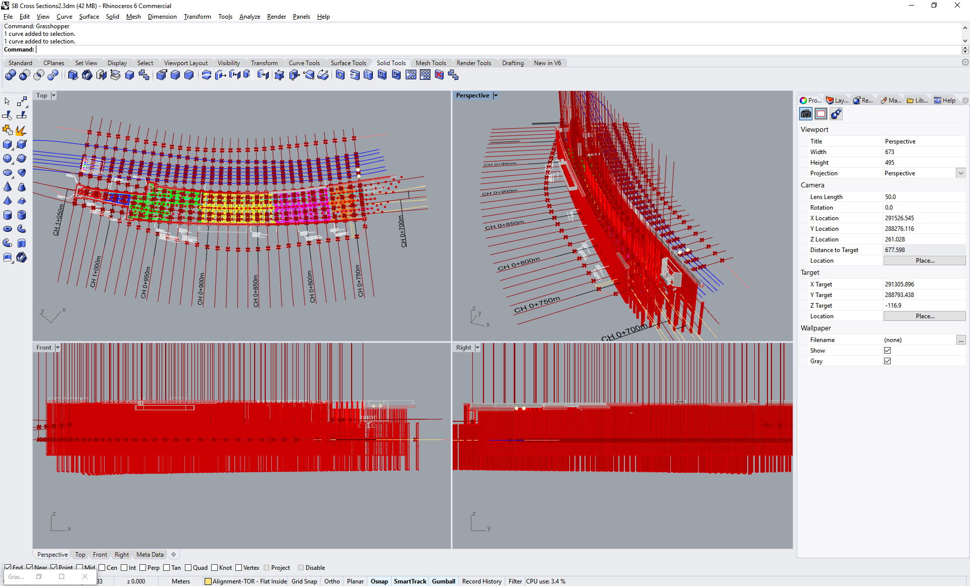
The 3D project BIM model is stored in a number of model files saved in the ProjectWise Common Data Environment (CDE) in Bentley Microstation (.dgn) format. The model files containing the main structural elements for the Euston Scissor Cut were imported into AutoCAD where additional information was added such as the location of the Park Village East retaining wall and Network Rail track alignments. The combined model was then imported into Rhino 3D as shown in Figure 2.

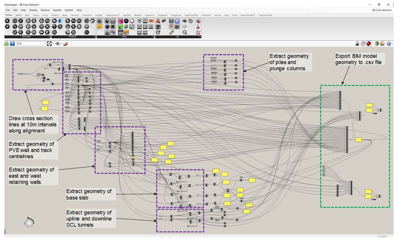
Rhino includes a visual scripting interface called Grasshopper, which was used to create cross section lines at 10m intervals perpendicular to the master alignment from chainage 0+750m to 1+040m along the length of the Euston Scissor Cut (30 sections in total). A Grasshopper script was developed (shown in Figure 3) to extract the plan coordinates of the key geometrical features (retaining walls, piles, plunge columns, HS2 tracks, Network Rail tracks) along each cross section line, as well as the elevation of the base slab, top of rail level and props.

Automation of Plaxis input

Plaxis 2D versions later the Anniversary Edition (AE) released in 2014^[2] include remote scripting API functionality that allows the user to interact with the program using Python coding instead of using the GUI.^[3] AutoPlx, a Python script previously developed by Arup, exposes the majority of the available Plaxis input and output API commands, with parameters read from an Excel file which exists in order to store them in a logical and checkable format. The script has been developed to set up and run multiple analyses consecutively, and can run in the background, on a remote desktop computer or can be left to run overnight, allowing the user to carry out other tasks while waiting for the analyses to complete.

As a validation exercise, a Plaxis section was manually set up using the GUI and then duplicated using the AutoPlx tool, with identical model setup, input parameters and results confirming the tool was performing as expected. The Euston Scissor Cut geometrical information, in tabular format as output from the Grasshopper script, was then added directly into a new worksheet in the AutoPlx Excel input file. The Excel VLOOKUP function was employed to read this table and populate the relevant fields elsewhere in the input file, depending on which of the 30 cross sections was currently being analysed.

As the design progressed, a number of additional details and sensitivity checks (such as construction loads applied at specific locations or variations in the assumed undrained shear strength of the soil) were added to the analyses. These additions were added as IF statements and VLOOKUP functions within the AutoPlx Excel input file rather than coding these into the Python script.

Extraction and presentation of results

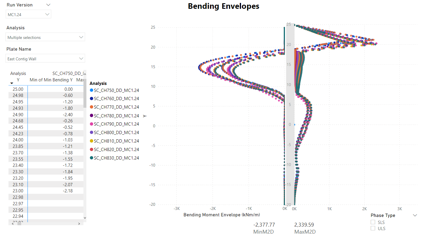
As well as allowing the automation of analysis set up and calculation, the Plaxis remote scripting API also permits the user to use Python coding to extract results at pre-selected construction stages and locations. Using this functionality, Python code was adapted to extract bending moment, shear force and displacement results for the Euston Scissor Cut retaining walls, piles and props, with the results stored in a comma-separated values (.csv) file.

Instead of manually setting up plots to present the results in Excel,^[4] a query was set up using PowerBI to automatically read all .csv files saved within the project directory. Automated calculations were set up within PowerBI to calculate envelopes of maximum and minimum results for each cross section, before the processed results were presented in a series of simplified visuals on a PowerBI report. The report was shared across the project team, with dropdown menu options allowing users to select and filter the results to view information for specific structural elements, construction stages or cross sections as appropriate. A page of the PowerBI report showing the retaining wall bending moment envelopes is shown in Figure 4.

Review of the Plaxis output in the PowerBI report allowed the critical cross sections through the Euston Scissor Cut to be identified, with additional optimisations and sensitivity checks targeting these locations then carried out by updating the AutoPlx input file and rerunning the Python script. The new results file was then added to the project directory and PowerBI query refreshed, automatically adding the results to the dataset and allowing the results to be viewed and compared to previous analyses in the PowerBI report.

Automation at Euston Crossover Tunnels and Euston Cavern

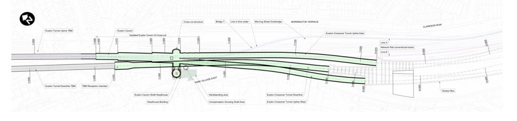
The Euston Crossover Tunnels and Euston Cavern serve as the transition from the twin TBM tunnels to the Euston Scissor Cut. The two TBM tunnels split into three sprayed concrete lining (SCL) tunnels and unwrap from a Downline-Upline-Upline configuration at Euston Cavern into the Upline-Downline-Upline configuration necessary for the switches at the Euston Scissor Cut (Figure 5).

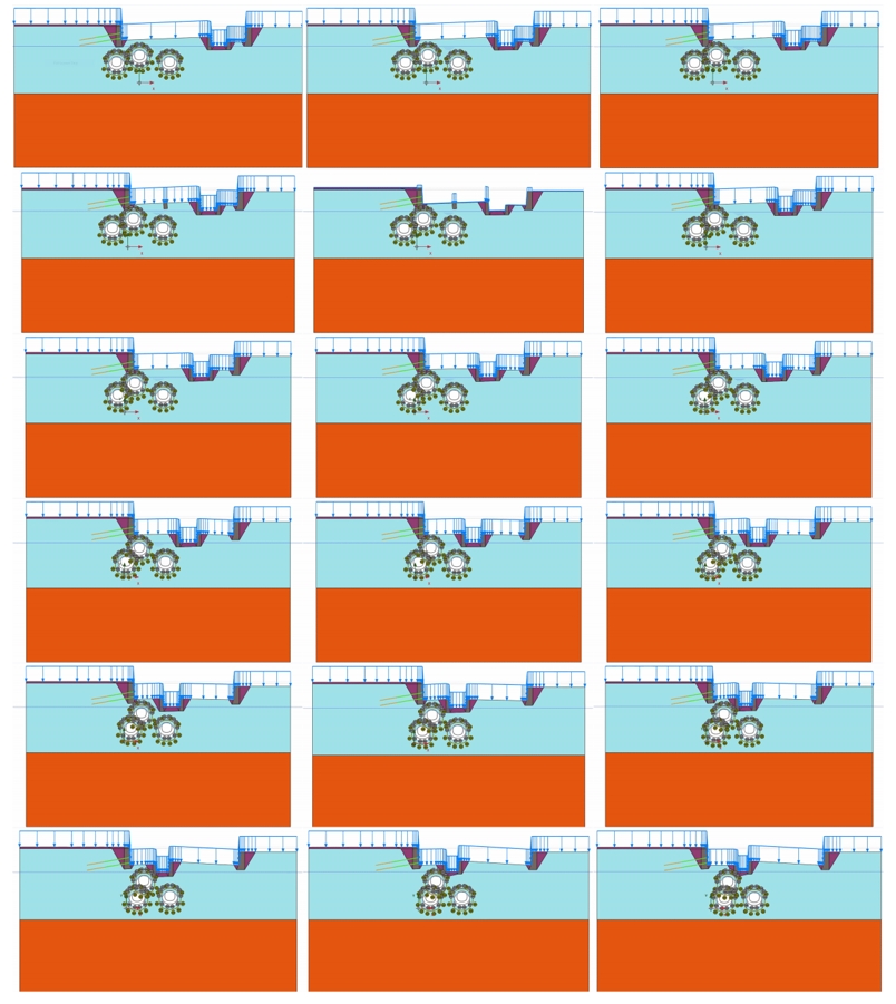
This unwrapping tunnel geometry is located under shallow ground cover beneath a complex arrangement of retaining walls up to 10m high. To perform the scheme design analysis, and later inform the ground movement assessment, many sections needed to be analysed to identify the critical sections and assess the interaction between the retaining walls and the SCL tunnels (Figure 6).

Typically, these models would be manually generated using a workflow similar to the following:

1. If a BIM model is available, ask for a cut to be generated at the required chainage.
2. Manually clean the exported DXF file for simplified input into Plaxis
3. By hand, assign material properties and materials to each area generated by Plaxis
4. By hand, generate staging for the rail cutting and tunnel excavation
   1. 1. To establish in situ stresses due to the rail cutting:
         • Initial grade
         • Excavation for retaining walls
         • Wall installation
         • Consolidation
         • Steady state groundwater regime
      2. For each of the three tunnels
         • Pilot relaxation
         • Pilot liner installation
         • Further relaxation and liner aging
         • Enlargement relaxation
         • Enlargement liner installation
         • Further relaxation and liner aging
         • Repeat
      3. Add any surcharge or point/line loading necessary for design
5. Extract results for each stage to assess the structural capacity of the tunnel liner.
   • Generate plots in Excel with Thrust-Moment interaction curves based on tunnel liner thickness/strength.
   • Manually match tunnel liner properties with stage results to assess based on modelled liner age/strength.

The workflow would need to be repeated for each new geometry and significant amounts of rework are necessary to assess changes in liner thickness, stiffness/strength gain or excavation sequencing. The manual workflow is also error prone due to the repetitive manual task of material properties definition, staging, and analysis options.

Early on in the scheme design it was identified that the manual process would not provide the level of quality or the quantity of analyses necessary for the structural design and ground movement assessments needed in the Euston Approach area. Working in collaboration with Arup, who funded the project, HS2 developed an alternative, automated approach.

Plaxis automation

Initially, the idea of Plaxis automation appeared straight forward:

1. Plaxis provides a Python^[5] API interface with some documentation,
2. (nearly) all commands entered into the Plaxis Graphical User Interface (GUI) are reproduced in the command shell, and
3. the sequence and structures of the Euston Approach do not significantly change, only their geometric arrangement.

Based on the above, if a single section of the Euston Approach could be automated, it should then be able to adjust the geometry of the retaining walls and tunnels to generate the models for the rest of the sections. This would mean that instead of needing to manually configure, analyse and post-process a dozen or more models, it could automatically configure, analyse and post-process a model every 10 metres.

The desire to limit repetitive manual tasks and to explore the benefits of automation led to the development of a Plaxis API Python high level wrapper called plxpy. A wrapper is software translation layer that streamlines common tasks but may not provide the full capabilities of the thing that it wraps. The development and use cases of plxpy are discussed below.

First Steps and Failures

To understand the commands that Plaxis requires to generate the models, the first task was to generate a simplified model by hand and try to re-create that model using the Plaxis API. Most of the geometry generation and naming conventions in Plaxis make sense:

• Every piece of geometry generated in Plaxis is assigned a name based on what order it was generated in
  • Polyline_1, Polyline_2
  • Line_1, Line_2
• The name of the generated geometry and any associated geometry are returned in the API call.
  • When Polygon_1 is generated, the polygon (Polygon_1 object) and the soil in the polygon (Soil_1 object) are returned.
• When a piece of geometry splits an existing piece of geometry, their names are derived from that split.
  • Where Polygon_1 intersects Polygon_2, Polygon_1_Polygon_2 is created.
  • Where Line_1 fully divides Polygon_2, Polygon_2_1 and Polygon_2_2 are created.

The above seemed promising, but there were still a few complications to address, that caused the task of automation to be more complicated than anticipated:

• The API is not designed to work outside of the Plaxis Python environment. It requires packages that are not publicly distributed.
• The geometry created before meshing is not the same as the geometry created after meshing.
  • Polygon_1 becomes Polygon_1_1
  • Line_1 may be divided into Line_1_1 through Line_1_5 due to intersections with other geometries along its length.
• Tunnels generated using the Plaxis Tunnel Builder tool do not respect the above conventions. The user cannot call “deactivate Tunnel_1 InitialPhase” to excavate the soil from the Tunnel_1. Soil polygons generated by creation of the tunnel are not associated with that tunnel.

Workaround for Tunnel Geometries

Because the SCL tunnels are the primary focus of the Euston Approach models and, as such, the limitations of the Plaxis API for tunnels needed to be solved. After several trial and error iterations, a fairly rigorous solution was identified that worked for all Plaxis geometries:

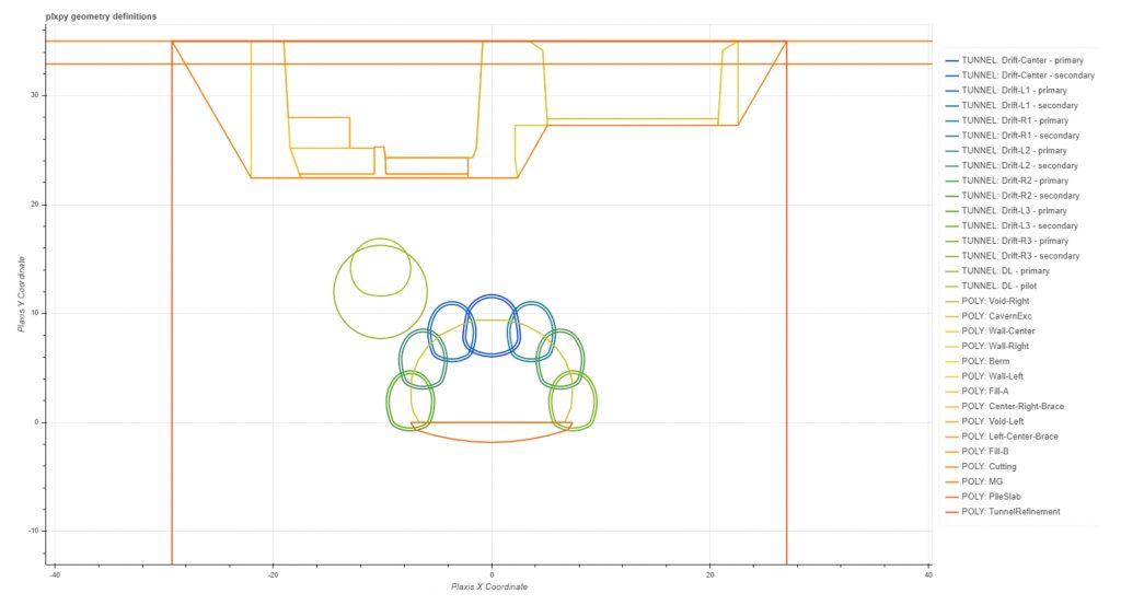
1. Based on user inputs, using a geometry workflow similar to those discussed for AutoPlx above, generate a Python geometry (Figure 7) and instruct Plaxis to generate each element of the geometry.
2. Generate the Plaxis mesh.
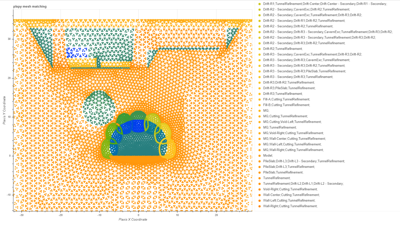
3. Extract the mesh nodes/interpolation points and match those points to the Python-geometry from Step 1.
4. Wherever the Plaxis mesh matches well (>99% of points matching) to the Python geometry, develop a mapping from the user generated name (e.g. Upline Tunnel) to the Plaxis geometry name(s) (e.g. SoilPolygon_1_2, SoilPolygon_3_2, etc.). An example of the matching results is shown in Figure 8.
5. Perform similar mapping between Python and Plaxis lines that are used to define ground anchor, wells, piles, etc.

Model definition

Apart from the difficulties associated with (hidden from the end user) geometry generation, the remainder of the model definition is straightforward. All inputs are provided in formatted text file similar to JSON that is interpreted by plxpy. For example, to define the stratigraphy the user would include the following block of text:

Stratigraphy:

Primary:

• [Ground_Surface, 35]
• [Ground_Surface, 35]
• [LC_Undrained, -5.0]
• [Lambeth_Group_Clay, -16.0]
• [Lambeth_Group_Sand, -25.9]
• [Thanet_Sand, -29.5]
• [Chalk, -45]

The soil unit names provided correspond to material property sets defined elsewhere in the input file and, by default, the units are horizontally bedded. Sloping stratigraphy is accommodated by adding addition offset borehole stratigraphies.

Staging definition is more complicated due to the detail necessary, but it generally simplifies down into a series of verbs and nouns. The user defines an action (e.g. activate, deactivate, change material, set pre-tensioning, etc.) and what object that action applies to (e.g. SoilPolygon_1_2, SoilPolygon_3_2, etc.). The created Python wrapper around the Plaxis API follows a similar syntax: the user specifies an action (verb) and then a list of objects (noun) that the action applies to. For example, to construct the retaining walls or excavate a tunnel the following instructions could be used. The stage name is italicised, verbs are bolded and nouns/settings are left in plain text.

Install PVE Wall:

ignore suction: true

use cavitation cutoff: true

cavitation stress: 100

max load fraction per step: 0.05

max steps: 10000

change polygon material:

• [Cutting, {to: Made_Ground_25deg}]
• [MG, {to: Made_Ground_25deg}]
• [Wall-Left, {to: Masonry}]
• [Wall-Center, {to: Masonry}]
• [Wall-Right, {to: Masonry}]
• [Left-Center-Brace, {to: Masonry}]
• [Center-Right-Brace, {to: Masonry}]
• [Berm, {to: Low_grade_concrete}]
• [Fill-A, {to: Made_Ground_25deg}]
• [Fill-B, {to: Made_Ground_25deg}]

activate polygon:

• Cutting

deactivate polygon:

• Void-Left
• Void-Right

activate polygon water, head:

• [Cutting, {head: 22}]

Cavern L3/R3 – 25% Relaxation:

m-stage: 0.25

ignore suction: true

use cavitation cutoff: true

cavitation stress: 100

max load fraction per step: 0.05

max steps: 10000

deactivate polygon water:

• D3L-Exc
• D3R-Exc

deactivate polygon:

• D3L-Exc
• D3R-Exc

Results extraction

After creating a solution to Plaxis automation using pure Python large portion of the modelling generation was able to be automated. This solved the time-consuming task of generating and executing models and shifted the focus onto results extraction and processing.

For tunnel liners, the focus of results, especially in the scheme and early detailed design, is on the structural behaviour of the liners. The tunnel liners can be modelled as either area or structural elements. Modelling as structural elements is simpler than using area elements, does not significantly increase the mesh size/runtime of the model and works satisfactorily for most cases. The results (thrust, moment, shear) are also easily extracted from the structural elements.

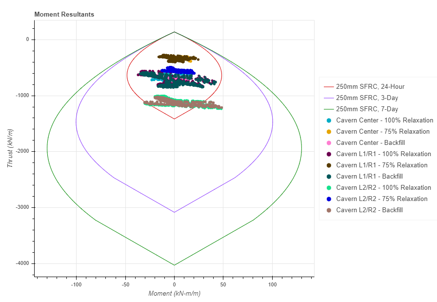
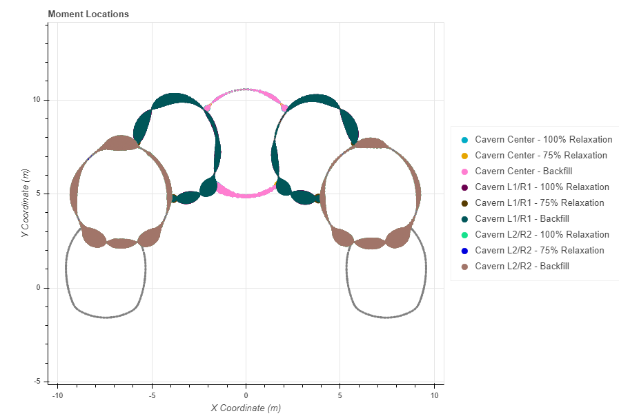
For the Euston Cavern – 15m Stacked Drift, the use of structural elements caused concern focused around the structural behaviour of the joint between adjacent drifts. The liners of all but the first drift were incomplete rings and relied on the end bearing/shear behaviour between the new liner and the in-place liner of the previous drift (note the C shaped liners shown in Figure 9). By modelling the tunnel liners as area elements the interface strength can be explicitly defined at the liner-liner joint (that also modelled as area elements) as well the tensile strength limit of the liner if interested in plastic liner behaviour.

The use of area elements can result in more challenging results extraction because the thrust, moment and shear are not an explicit result (such as for a plate element) but are a result of stress integration across the section thickness. Plaxis provides an interface for defining an area element centreline and automatically performing the stress integration to determine the equivalent moment, thrust and shear. A wrapper for this interface has been included in plxpy. The wrapper allows the user to request results for multiple centrelines and multiple stages with results returned as a pandas^[6] DataFrame.

The results returned can then be plotted against their position to allow a detailed inspection, and design against, the moment-thrust interaction results (Figure 9 and Figure 10). The two plots shown in Figure 9 and Figure 10 are generated using Bokeh^[7], with a dynamic link between plot panes so the user can lasso-select a cluster of points on the interaction diagram to show where they are physically located (the reverse operation is also supported).

Conclusion

The case studies presented in this paper show that the automated approach to setting up, running and reviewing 2D FE analyses have led to a number of benefits in the design process. While time consuming to initially learn how to use the Plaxis API and adapt existing Python coding to meet the needs of the HS2 Project, the reduction in the number of manual steps typically required when running FE analyses allowed an increased number of analyses to be carried out. This meant that instead of having to identify the critical locations at which to carry out analysis in advance, many closely spaced cross sections were analysed and the critical locations identified by inspection of the results. Sensitivity checks were then carried out by varying key design input assumptions such as soil strength to ensure that the design outcome was appropriate.

This automated method also allowed Plaxis to be extended through Python coding to run analyses with much more complicated geometries than can typically be carried out when interacting with the program manually. By automating the input, analysis and extraction of results, the risk of human input error is also reduced, while the process of checking is also streamlined through being able to review both the program input parameters set out in a tabular format in the Excel input file, as well as being able to compare the output from multiple analyses side by side in PowerBI.

Drawbacks to automating FE analysis exist however, including the computing resources, use of software licences, the long duration to run and the large amount of data returned from running numerous analysis. This needs to be well managed, including establishing naming conventions for files and construction stages, as well as setting up analyses to run overnight when demand for software licences from other users is less. The automated approach also requires the BIM model to be well developed at early design stage which is not always the case as the BIM model typically develops in tandem with the design.

In conclusion, it is recommended that geometrical information is modelled in BIM as early as possible, with automated design activities based on this initial geometry then carried out. Once refined design output becomes available, this should then be fed back into the model and design calculations updated. There are still several manual steps in the processes described in this paper, such as manually exporting the BIM model, adding additional information and importing into Rhino, or making Plaxis output available for import into PowerBI. These steps should be automated in future to refine the process further.

References

1. Bond, A.J. and Harris, A. (2008) Decoding Eurocode 7, London: Taylor & Francis.
2. Plaxis (2014) New Release: PLAXIS 2D AE, accessed 23 July 2020
3. Plaxis (2015) Using PLAXIS Remote scripting with the Python wrapper, accessed 23 July 2020
4. Microsoft (2020) Six ways Excel users save time with Power BI, accessed 23 July 2020
5. Van Rossum, G., & Drake, F. L. (2009). Python 3 Reference Manual. Scotts Valley, CA: CreateSpace.
6. McKinney, W., & others. (2010). Data structures for statistical computing in python. In Proceedings of the 9th Python in Science Conference (Vol. 445, pp. 51–56).
7. Bokeh (2020). Bokeh: Python library for interactive visualisation.