Overcoming the challenges associated with the design of noise barriers for High-Speed Railways
Noise barriers on high-speed lines have attracted significant attention in recent years due to concerns over performance in use. Lightweight barriers have been damaged by bird strike, train aerodynamic pressures have led to some early fatigue failures and materials selection with limited durability have led to unexpected maintenance costs.
This paper presents the results of dynamic analysis to meet the requirements of BS EN 16727-2-2: 2016 for HS2, including a determination of the dynamic response of noise barriers. It considers variations in both the modal properties of the barrier and the spectral content of the train pressure loading, and considers cumulative effects from the nose, inter-car and tail pulses.
The relationship between the spectral content of these pulses, along with the main response modes of the barrier is demonstrated graphically in order to clarify the response peaks which should be designed for or avoided.
Design solutions for these peaks are explored including damping and strengthening solutions, along with confirmation by testing.
The design is based around a cranked noise barrier geometry selected for visual impact and acoustic reasons and consistent with the emerging Common Design Element (CDE) proposals. This introduces additional complications over traditional vertical barriers which are also highlighted in the paper.
- Written by
-
Rory Bradshaw (SCS/Arup)

-
Faraz Ul-Haq (SCS/Skanska)

- Resource type
- Resource type: Technical Paper
- Tags
- dynamics posts
- fatigue posts
- High speed posts
- Noise barriers posts
Introduction
This paper presents work completed to develop the design of noise barriers at West Ruislip on the southern section of High Speed Two (HS2) Phase One – Lots S1 and S2 (Area South) which includes the Northolt Tunnels and the Euston Tunnel and Approaches being delivered by the SCS Integrated Project Team.
The design of the noise barriers accords with the emerging Common Design Element (CDE) proposals for lineside noise barriers presented to the Phase One Planning Forum. The noise barriers have been conceived to provide a high-quality design that contributes to the HS2 route-wide identity and sits comfortably within the family of other CDEs whilst maintaining the flexibility to meet differing acoustic requirements
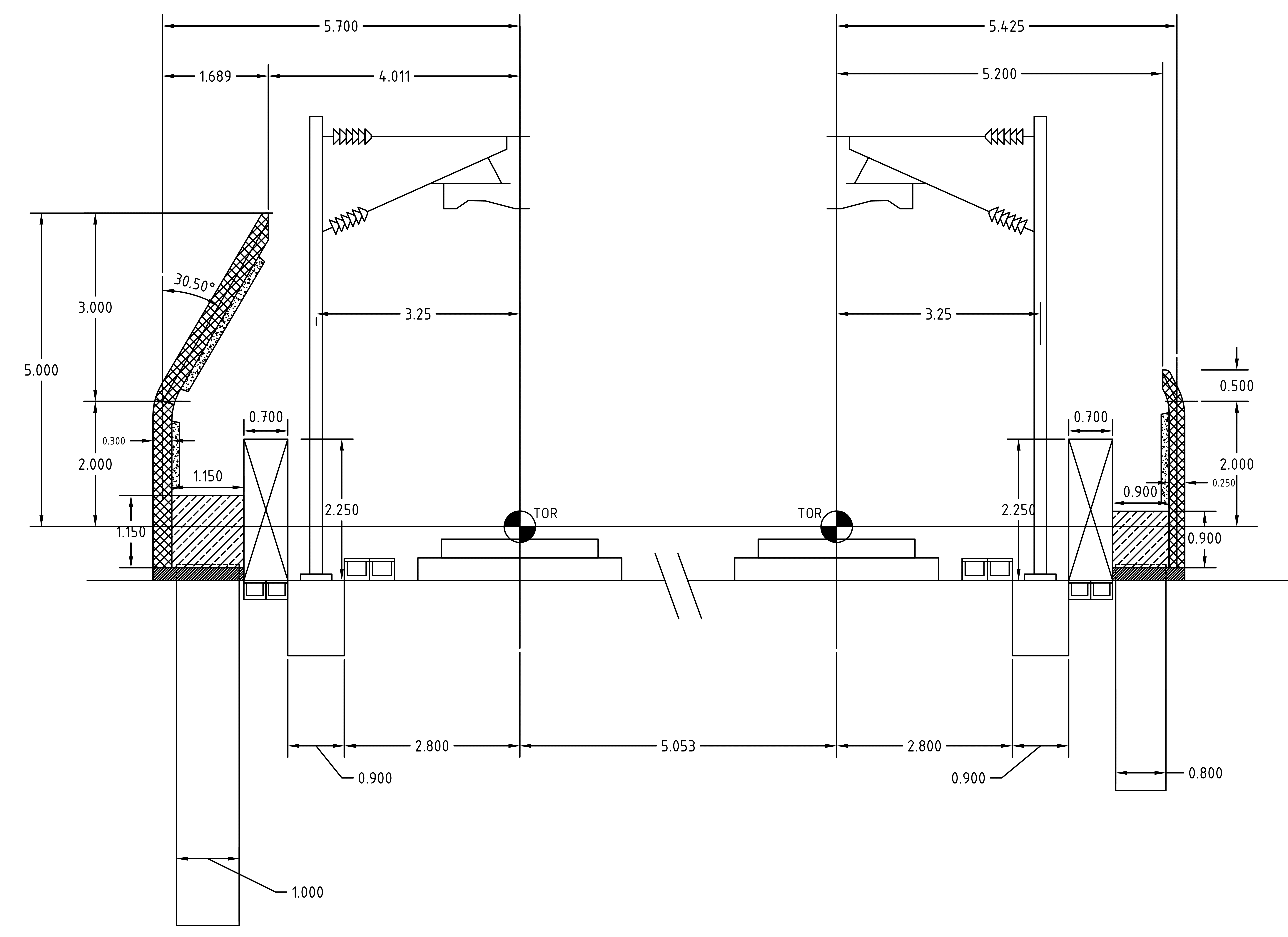
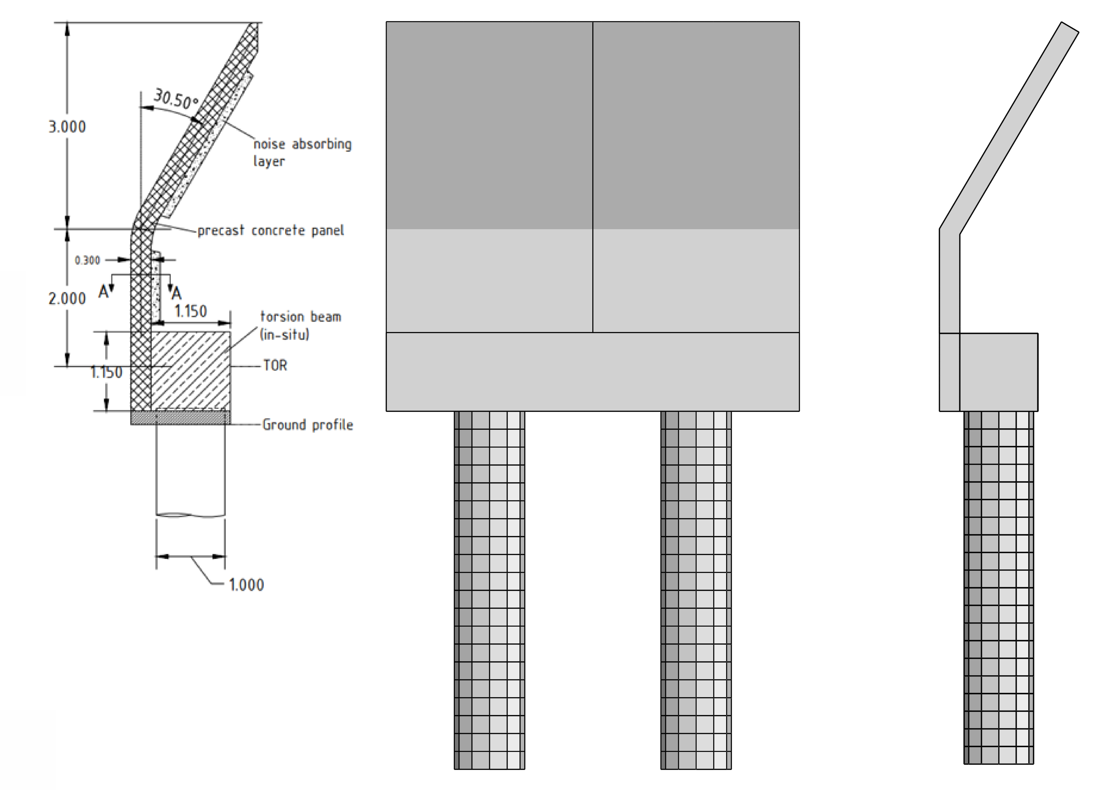
A typical section of the track is shown in Figure 1. This shows a cranked noise barrier of height just over 5 m (5 m above TOR) which is adjacent to the down-line and lies to the south-west of the line. A shorter vertical noise barrier is also shown adjacent to the up-line. This paper will focus on the taller cranked barrier, though the same principles highlighted in this paper are equally applicable to the shorter vertical noise barrier. An important constraint on the design was that any posts, if used to support the barrier, should not be visible on the outside.
The cranked barrier panels are supported by a 1.15 m square “torsion beam” which runs parallel to the track and transfers moment from the panels to the piles in torsion.
The cranked barrier was arrived at after considering several noise barrier options evaluated against a range of criteria including the predicted acoustic effects, landscape and visual effects, engineering practicability and value for money. The preferred option of the cranked barrier was selected on the basis that it reduced noise as far as reasonably practicable and represented the optimum balance between maximising the acoustic benefits, whilst minimising visual impacts. A tall vertical face, often presented by conventional noise barriers, may have seemed abrupt in the context of the contours of a natural landscape and the strong horizontal of the railway corridor. By cranking barrier and creating a receding visual form, the barrier design achieved an efficient acoustic solution which is more sympathetic to its surroundings.
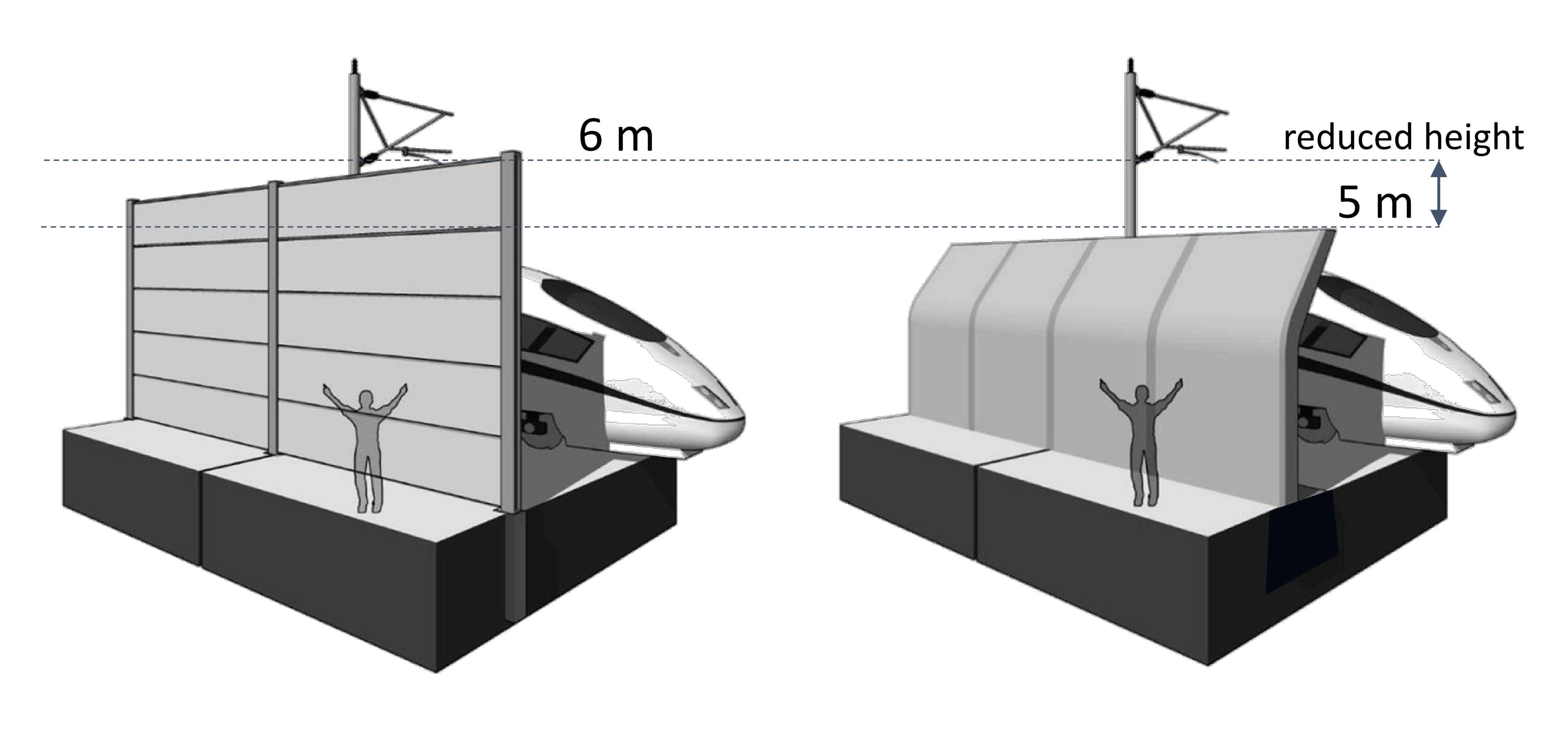
Due to the increased acoustic efficiency, the crank allowed a shorter barrier for the same acoustic performance. With this in mind a 5 m high cranked barrier is contrasted with a 6 m high straight barrier in Figure 2 in order demonstrate the possible visual benefits of the crank. It should be noted that the crank did pose challenges in design and these will be described in this paper.
The paper will describe the main structural challenges of design and associated loading models for the barrier. Load models will be reviewed at a high level with a traditional shock-spectrum approach using a 1 degree-of-freedom (1-dof) system, prior to the presentation of finite element analysis results explaining:
- some options ruled out and why;
- the complications with the crank;
- the potential danger of using dynamic amplification factors (DAFs) in design;
- the possible benefits of changing the frequency of the barrier or its damping;
- the significant amplifications at the ends or barrier and how this was avoided.
Finally, the paper summarises testing planned for the noise barriers.
Design of Noise Barriers for Pressure Loading
The Pressure Pulse
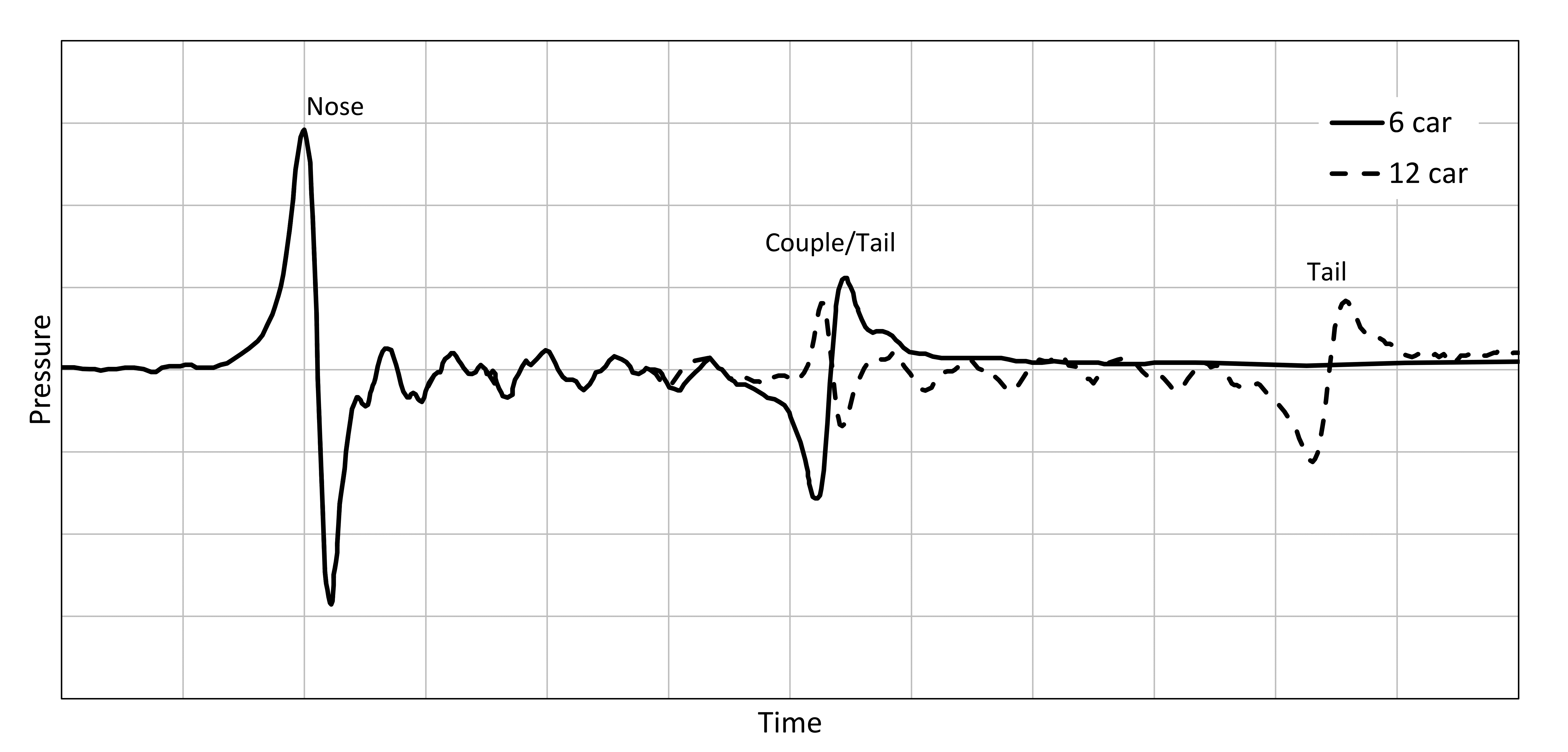
As a train moves along the track there is a pressure field in the air around it which is carried along with the train. Pressure changes are caused by the train pushing air out of its way, and the air moving back after the train passes. A structure near the track experiences a pulse of positive pressure then negative pressure (suction) as the nose passes. Similar pulses occur at the tail of the train and at the coupler where two trains are coupled together (for example when two no. 200 m trains are coupled together on HS2 to form a 400 m train). Smaller pressure pulses are caused by the inter-car gaps, though the latter tend to have a less clearly defined shape compared to the nose, tail and coupler pulses. The pulse at the nose is illustrated in Figure 3 and a measured pressure shape is shown in Figure 4.
The combined effect of the push-pull nature of the pressure distribution from the nose, followed by a similar loading event from the rear of the train a short time later, can lead to large dynamic effects and fatigue damage.
This loading has led to fatigue failures in Germany[1].
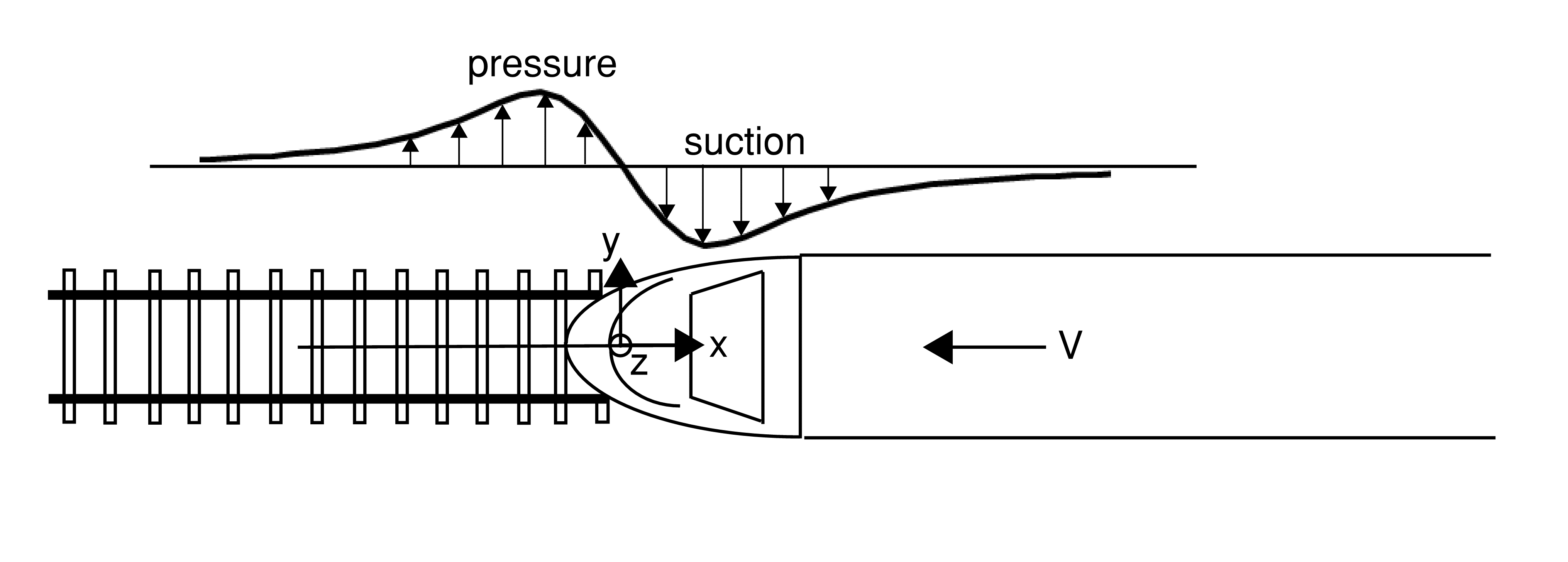
Note: the pulse shown is not to scale. The actual pulse drawn would be over a total length of circa 80 m
Codes and Papers on Designing Noise Barriers
Most European codes use a pressure pulse which is rectangular[3][4][5][6][7] and are intended to be used as part of a pseudo-static design process with a DAF. These do not resemble real pressure pulses such as those shown in Figure 4.
Significant factors relevant to designing a noise barrier were considered to be the:
- peak pressure on the barrier;
- reduction in peak pressure with distance of the barrier from the track;
- reduction in pressure with height up the barrier;
- adjustment to pressure for cranked barriers;
- existence of a dynamic load model.
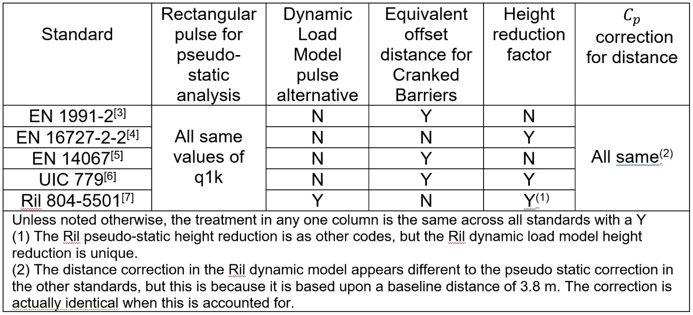
A review of how codes cover these factors is summarised in Table 1 for the Eurocodes, UIC 779 and Ril 804. The following observations can be made:
- All codes determine the peak pressure the same way for pseudo-static analysis (though dynamic amplification and subsequent use of these values does differ).
- The treatment of height reduction and cranked barriers is not covered consistently. Only the UIC covers both.
- The Ril standard includes a full dynamic load model developed in response to noise barrier failures in Germany[1].
- EN 16727-2-2 requires an appropriate load model for barrier design when not following the pseudo-static approach.
HS2 has developed guidance on the aerodynamic loads for the design of noise barriers. These advises the use of either a simplified triangular load model or the Ril load model. Both have been considered in design and are under discussion with HS2.
Other useful information and guidance can be found in Lachinger et al[8], Belloli et al[9], Tokunaga et al[10], Friedl et al[11], Hoffmeister[1] and Baker et al [12].
The Dynamic Load Models of HS2 and Ril 804
As summarised above, a dynamic load model is included in the Ril 804 but not in the other codes considered.
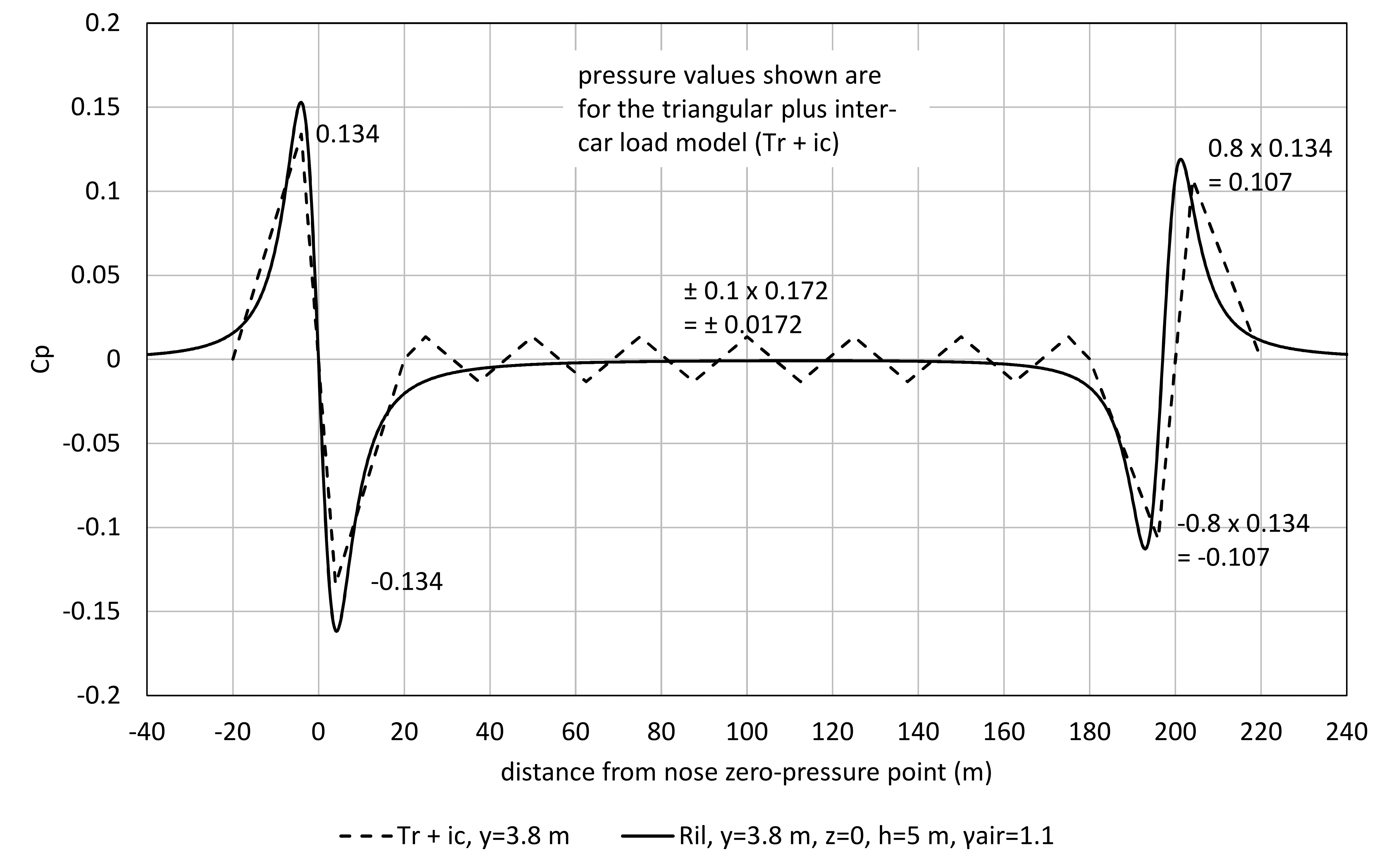
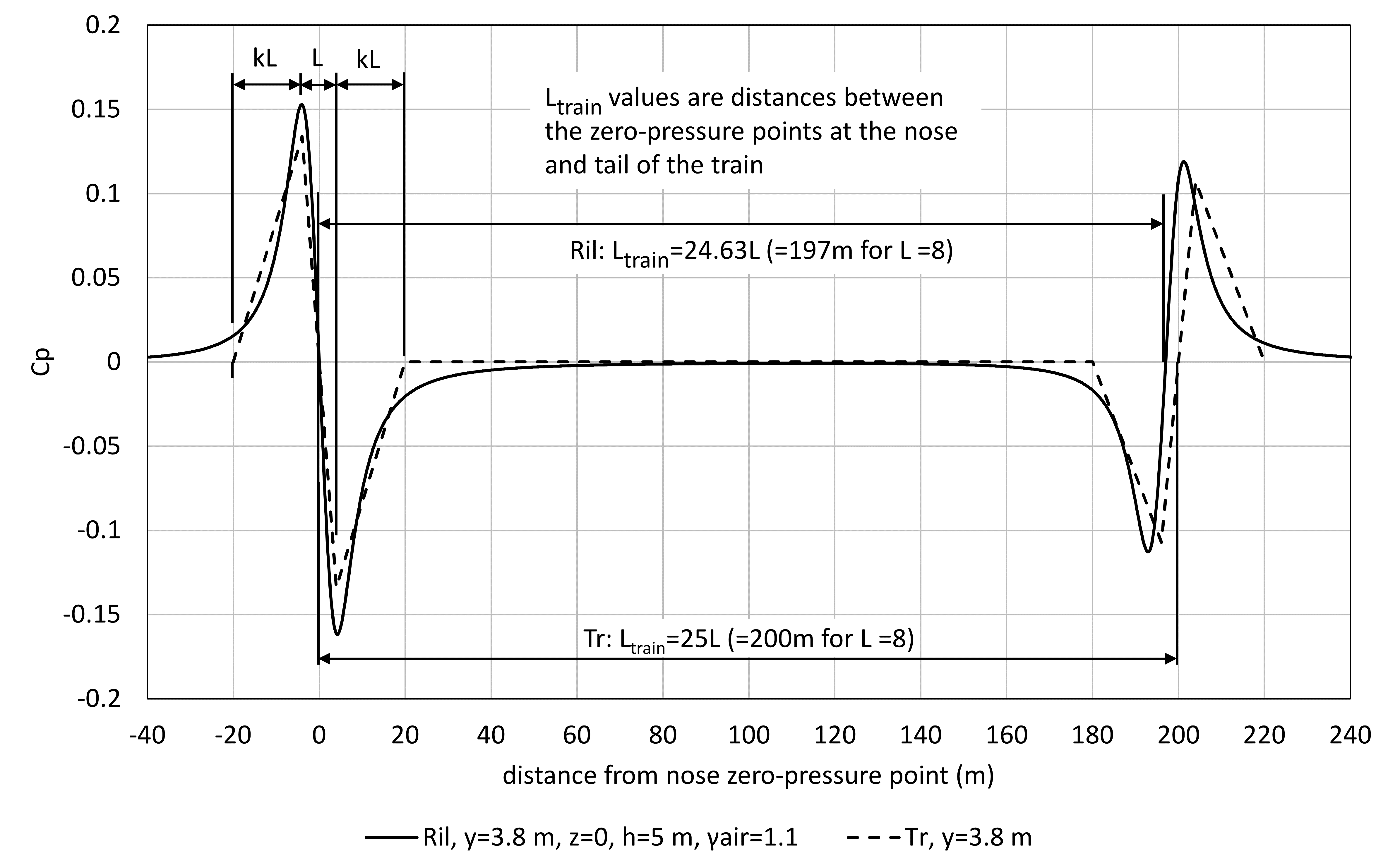
A simplified load model has been development by HS2 and this is shown in Figure 5 for a 200 m train along with the corresponding Ril load model for a barrier that is 3.8 m from the centreline of the track and 5 m high. The length parameters for the nose pulses and spacing between the nose and tail are also shown in Figure 6 (excluding the inter-car pulses of the HS2 load model for clarity). Note that:
- L = 8 m for both the HS2 and Ril load models.
- The factor k is a variable in Figure 6, though it was fixed at 2 in the HS2 load model. The factor k is only relevant to considering variations in the HS2 load model.
- Both load models contain a larger nose pulse, followed by a tail pulse around 200 m behind.
- The distance between the zero-pressure point of the nose and tail pulse
 is slightly different between the two load models.
 - The value of
 in Figure 5 is converted to pressure at the level of the TOR as in Equation (1).
 - The HS2 load model does not depend upon the height of the barrier but the Ril does.
- The HS2 load model does not have a reduction in pressure with height up the barrier. The Ril load model does reduce pressure with height, so the Ril plot would be smaller than the HS2 further up the barrier. Consequently, although the HS2 pulse peak value is below the Ril pulse in Figure 5, the static value of base moment from the HS2 pulse is close to that from the Ril pulse in this case.
- The HS2 load model explicitly includes inter-car pulses along the train which are 10% of the magnitude of the nose pulse, spaced at 25 m (or 3.125L in normalised form). The Ril load model does not explicitly include inter-car pulses.
As the HS2 load model is made from triangular wave forms and has inter-car pulses it is referred to for brevity as “Tr + ic” or “Tr” when the inter-car pulses are excluded. Note that the Tr load model is hypothetical and is simply used as a “stepping-stone” to help compare the Ril and Tr + ic load models.
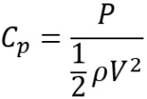
In this paper the pressure coefficient ![]() is the ratio of the highest pressure in the load model to the Bernoulli pressure as shown in Equation (1) where
is the ratio of the highest pressure in the load model to the Bernoulli pressure as shown in Equation (1) where ![]() should be taken as 1.25 kg/m3.
should be taken as 1.25 kg/m3.
It should be noted that the Ril code includes a ![]() term of 1.1 to include for variation in air density which is separated from the
term of 1.1 to include for variation in air density which is separated from the ![]() value. However, in this paper the 1.1 factor is included in the
value. However, in this paper the 1.1 factor is included in the ![]() value to allow for direct comparison between
value to allow for direct comparison between ![]() values of different load models.
values of different load models.
In the Tr + ic load model, the peak value of Cp is simply:
(2) ![]()
where
(3) 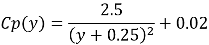
and
y is the distance from the centre of the track to the barrier
0.6 is a factor for streamlined HS trains (e.g. ETR, ICE, TGV, Thalys, Eurostar or similar). This was assumed for both the HS2 captive and classic compatible trains.
1.3 is a factor for localised peak pressures.
For y = 3.8m this gives
(4) ![]()
Hence, ![]()
The peak values of ![]() for the rest of the Tr + ic load model are determined from this value as shown in Figure 5.
for the rest of the Tr + ic load model are determined from this value as shown in Figure 5.
The pressure at the base of the Ril model is barrier-height dependant and it is worth noting that the peak pressure values would be significantly reduced with shorter barriers.
Dynamic Analysis of a 1-DOF System
It is possible to get some insight into the two loading models by considering the response of a one degree of freedom (1-dof) system to the load models.
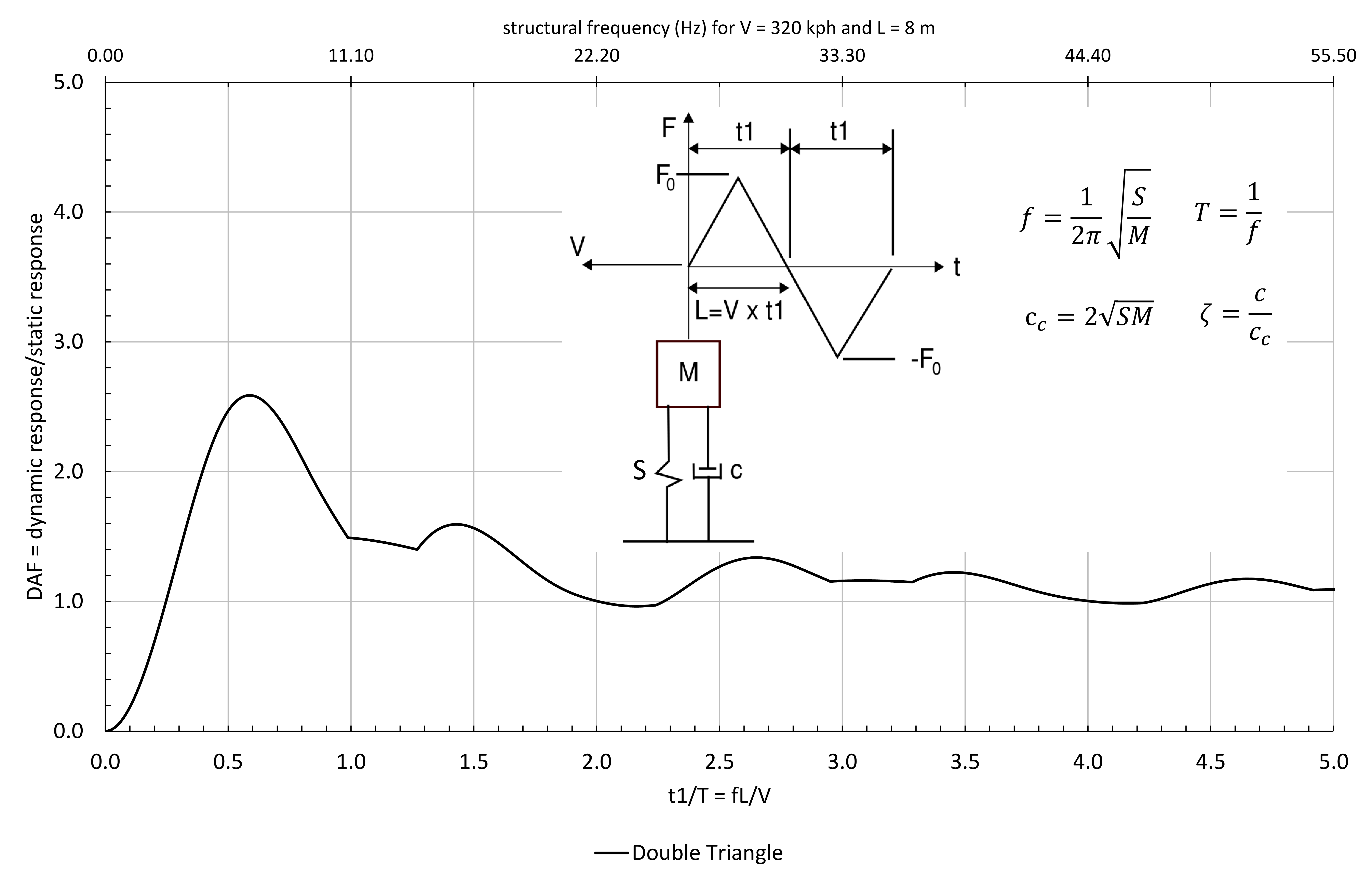
A 1-dof system is illustrated in Figure 7. This consists of a mass on a spring of stiffness S (N/m) and dashpot damper of viscous resistance c (N/(m/s)) giving a damping ratio. A force in the form of a double-triangular pulse, with each triangle of characteristic length, L, can be imagined moving over the mass at speed V, so on a time axis, each triangle has a duration of t1 = L/V. The dynamic response can be obtained using, for example, Duhamel Integrals (see Harris and Crede[13]) or explicit time integration (see Bathe[14] ). From this analysis the peak dynamic response of the system can be obtained (Xmax).
The DAF is then defined as:
(5) ![]()
where:
(6) ![]()
and F0 is the maximum value of the force in the time history of applied loading. The standard shock spectrum for this pulse is also shown in Figure 7 which shows a maximum DAF of 2.6 at the critical value of f L/V of 0.6.
Using a similar principle, the normalised shock spectrum for the load models shown in Figure 6 can be seen in Figure 8 for the Ril pulse and for the Tr pulse (for k = 0.75, 1.25 and 2) for a damping level of 1%. For convenience an additional axis has been added to the top of the normalised shock spectrum showing the frequency of the structure for V = 320 kph and L = 8 m.
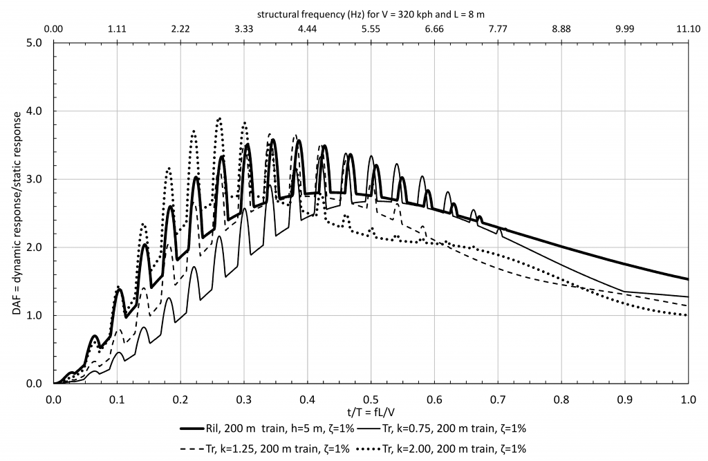
As both load models lead to a similar static moment at the base of the barrier, the DAF gives a good indication of the relative impact of each load model on design.
A number of significant observations can be made from Figure 8.
- The response is characterised by a hill with several spikes on the hill. The peak values of response tend to be in the region of f L/V from 0.25 to 0.5. This corresponds to a structural frequency range of 2.8 Hz to 5.6 Hz for V = 320 kph and L = 8 m.
- The nose pulse in isolation was found to be the cause of the main hill, whilst the tail pulse caused the spikes on the hill.
- The spikes on the hill were found to be caused by the tail pulse arriving at the right time to have maximum additive effect to the vibration remaining from the nose pulse. The maximum DAF is 3.9 at f L/V = 0.26.
- On the normalised horizontal axis, the distance between the peaks is L/Ltrain and each spike occurs at (n + 0.5)L/Ltrain where n is an integer representing the number of oscillations of the barrier between the arrival of the nose pulse and the tail pulse.
- The hill of the Ril is wider than the hill for each Tr response. By inspection, the Ril load model (see Figure 5) has a smooth transition of curvatures (similar to measured pulses such as in Figure 4) which suggests a broad spectral content compared to the Tr load model. As the Tr load model is more spectrally focused, it appears to be necessary to consider a range of k values in order to obtain higher responses over a broader range of f L/V.
- When k = 2 the Tr pulse is close to or above the Ril pulse up to f L/V = 0.35 (or up to a structure with a maximum natural frequency of about 3.9 Hz for V = 320 kph and L = 8 m).
- For any one value of k, the response to the Tr load model can lie significantly below that from the Ril for some f L/V. To avoid unconservative results (relative to the Ril) a range of k values is therefore necessary. In order to make the Tr pulse close to or above the Ril for up to f L/V = 0.60 it appears to be necessary to have a range of k values from 0.75 to 2.00
The same plot is also shown in Figure 9 for the Ril and Tr + ic load models. This leads to the same comments as above except that it is noted that the Tr + ic pulse has some significant spikes above the Ril at f L/V less than about 0.3 with a DAF reaching 4.8 on the highest spike at f L/V = 0.3.
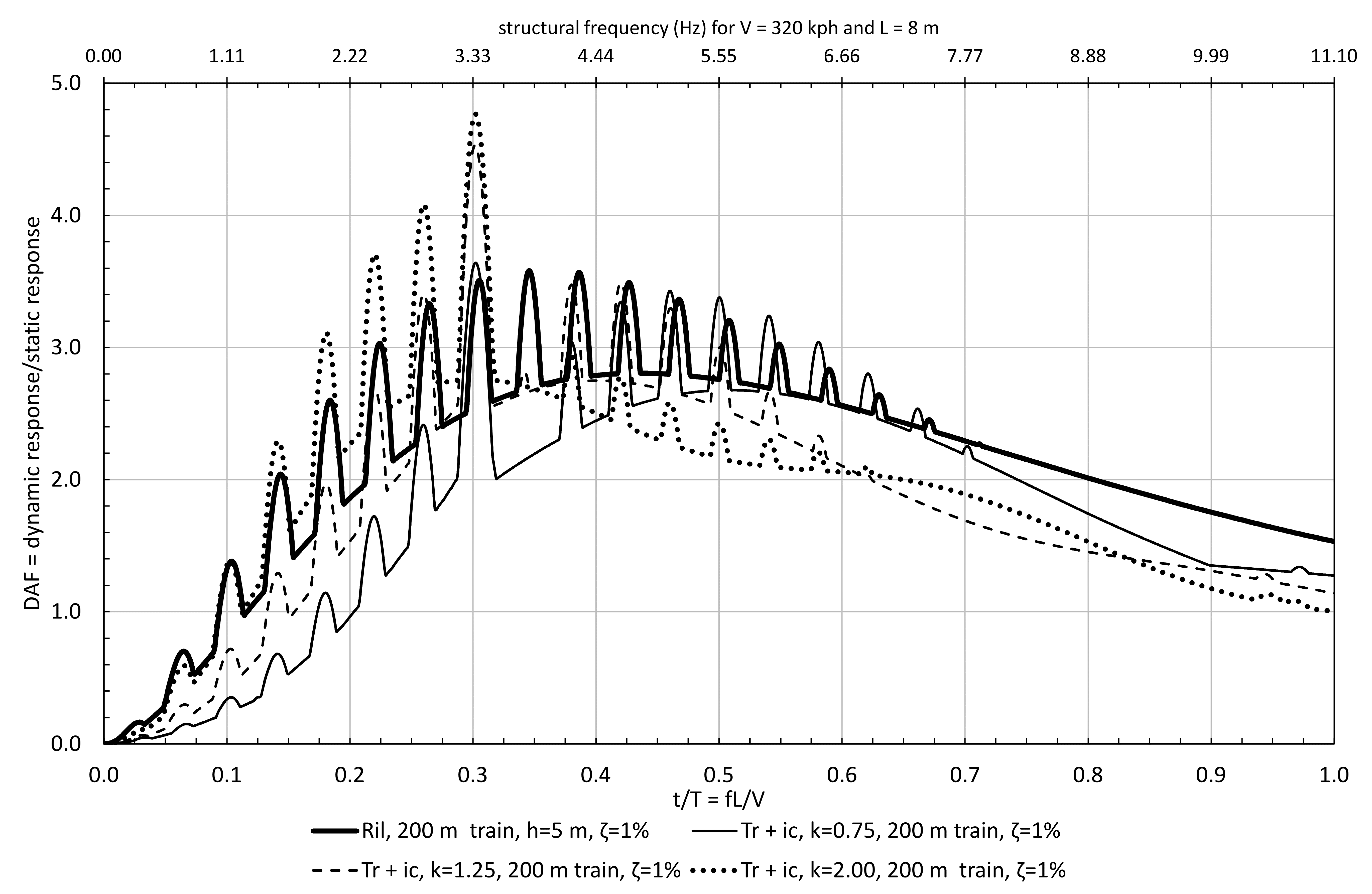
It may be easier to visualise the significance of this in non-normalised form; consider inter-car pulses spaced at 25 m travelling at 88.89 m/s. Resonance would occur on a structure of natural frequency 88.89/25 = 3.56 Hz. This is at f L/V = 3.56 x 8 / 88.89 = 0.32 which is close to the peak observed above. In normalised form the same value is simply arrived at as L/25 = 8/25 = 0.32.
The increased peaks from the inter-car pulses are caused by resonance, and they lead to an increase of 4.8/3.9 = 23% comparing peak values of DAF of Tr + ic with Tr.
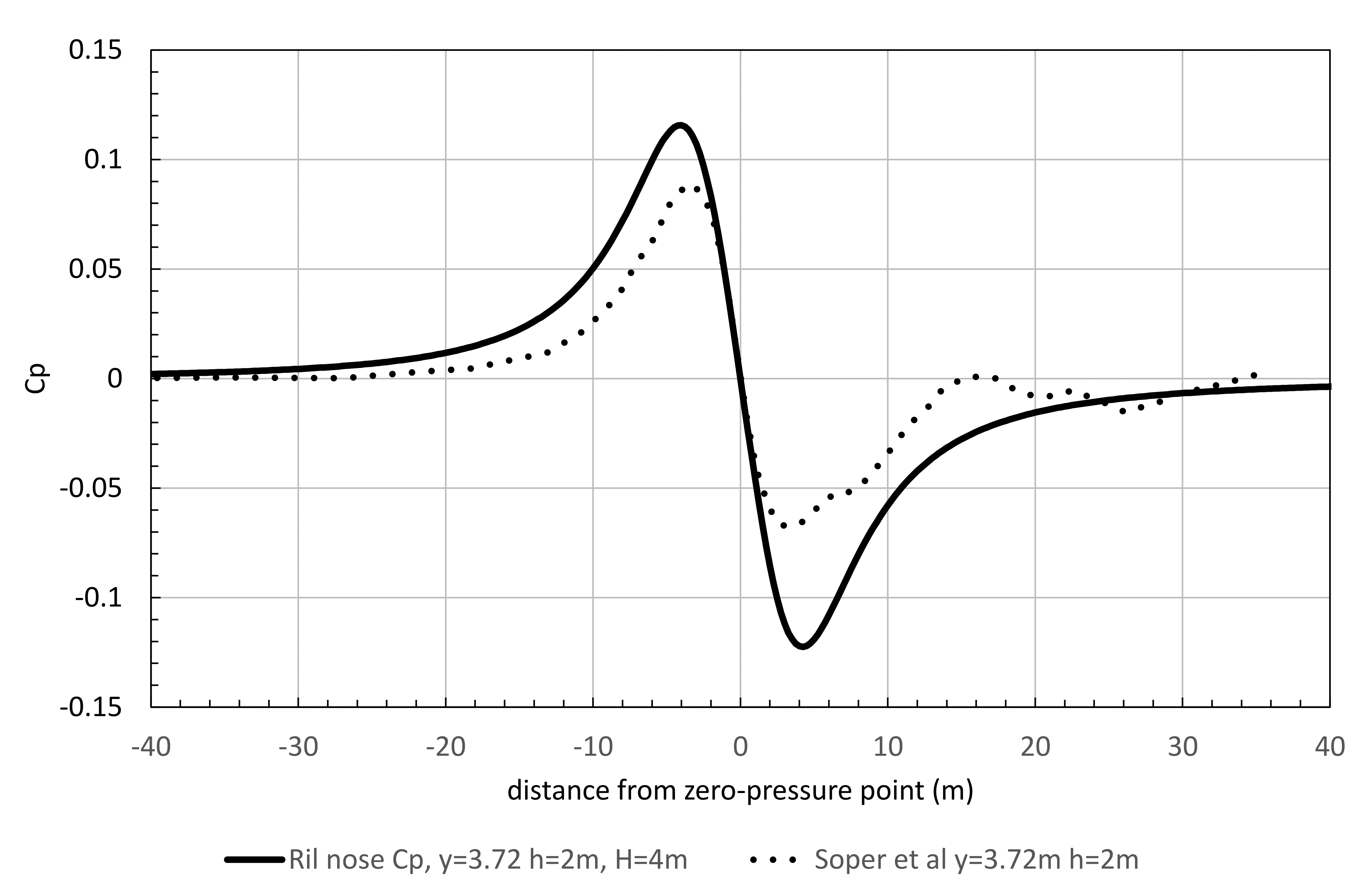
The Ril nose pulse is compared to an ensemble (mean) of results presented by Soper et al[2] in Figure 10. The Ril nose pulse is greater than the ensemble of results by about 30% on positive C_p values (0.12/0.09 = 33%). It is therefore possible that the Ril pulse may have been scaled up to include some effect of inter-car pulses. It is also worth noting that real inter-car pulses are not so regular as the triangles in the Tr + ic load model (see Figure 4) so the level of resonant build-up would be less in practice than that predicted by the Tr + ic.
These results are under review with HS2 for future research purposes and for the development of load models.
Reducing Structural Response
It is clear from the plots presented that a shift in stiffness or mass to make f L/V greater than about 0.6 (or f > 6.66 Hz for V = 320 kph and L = 8 m) could lead to a significant reduction in DAF. This may be practical in some situations, though it may be difficult to achieve in practice for tall concrete barriers. The introduction of significantly lighter steel or aluminium in-fill panels could facilitate this shift of frequency. However, experience on HS1 and other high-speed railways (with lower traffic than HS2) has shown up other fatigue, durability and robustness issues with lighter panels.
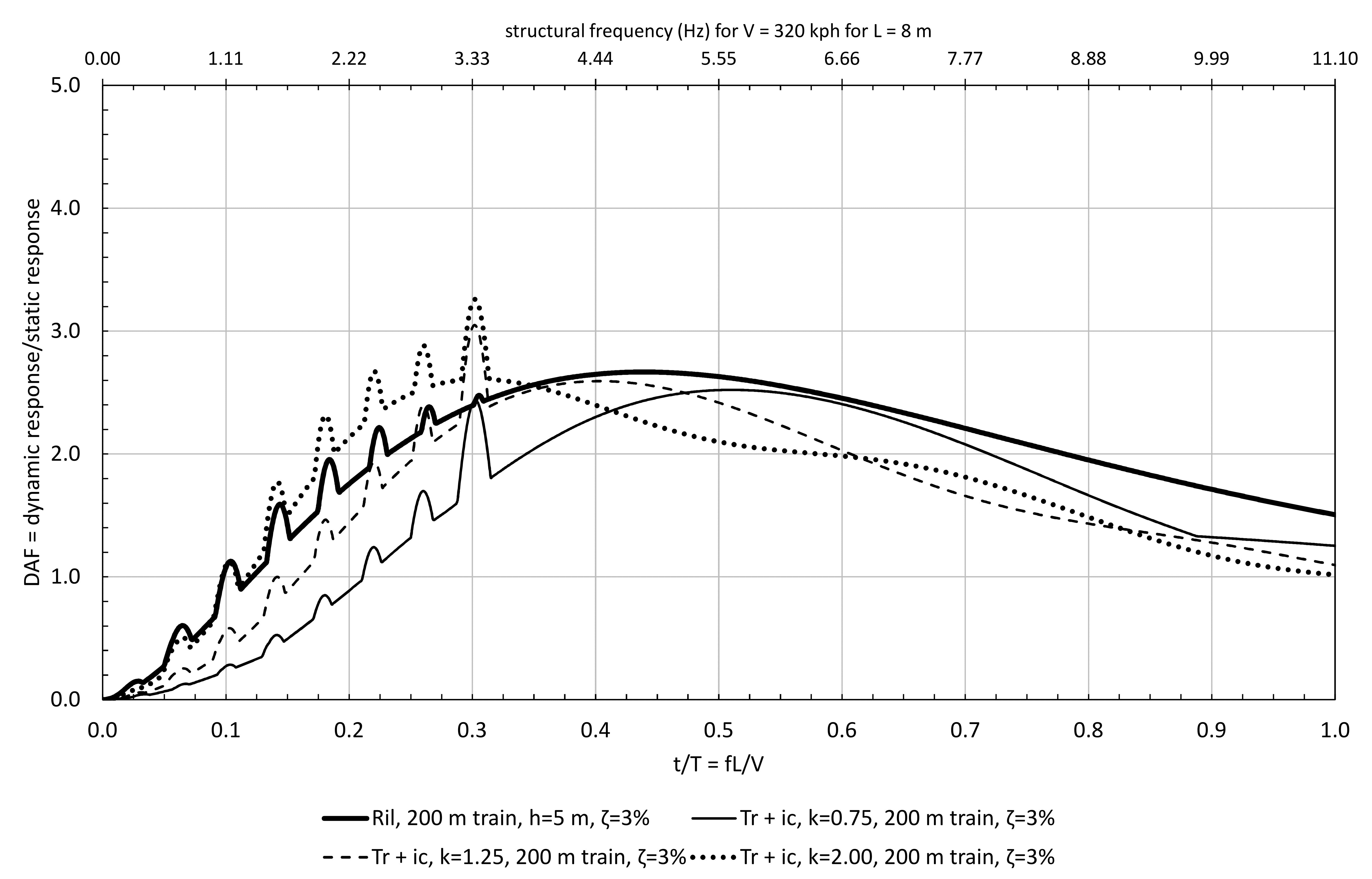
When the damping was increased to 3% there was a significant drop-off in response as shown in Figure 11. The extra damping had little effect upon the nose pulse (the main hill) but did significantly reduce the effect of the tail and inter-car pulses. The damping of a barrier is site dependant and it is difficult to avoid a conservative value in design without early testing. Tuned mass dampers (TMDs) were considered to provide damping but were ruled out as the amount of tuning involved was considered impractical. Also, TMDs would have introduced a maintenance overhead.
With all the above taken into consideration (particularly the planning constraints), it was decided to design for the loads where the structure naturally fell on the f L/V axis and with codified values of damping.
Arrival at the Torsion Beam Option
A common approach to noise barrier design uses steel H-posts with concrete planks or panels fitted between the flanges using elastomeric strips to avoid high stresses and provide damping. This type of design is described and included in most standards on noise barriers.
Due to the cranked geometry needed at West Ruislip, this typical design was not an option. The crank meant that planks could not be inserted from the top and planning considerations at West Ruislip required that posts would not be visible on the outside.
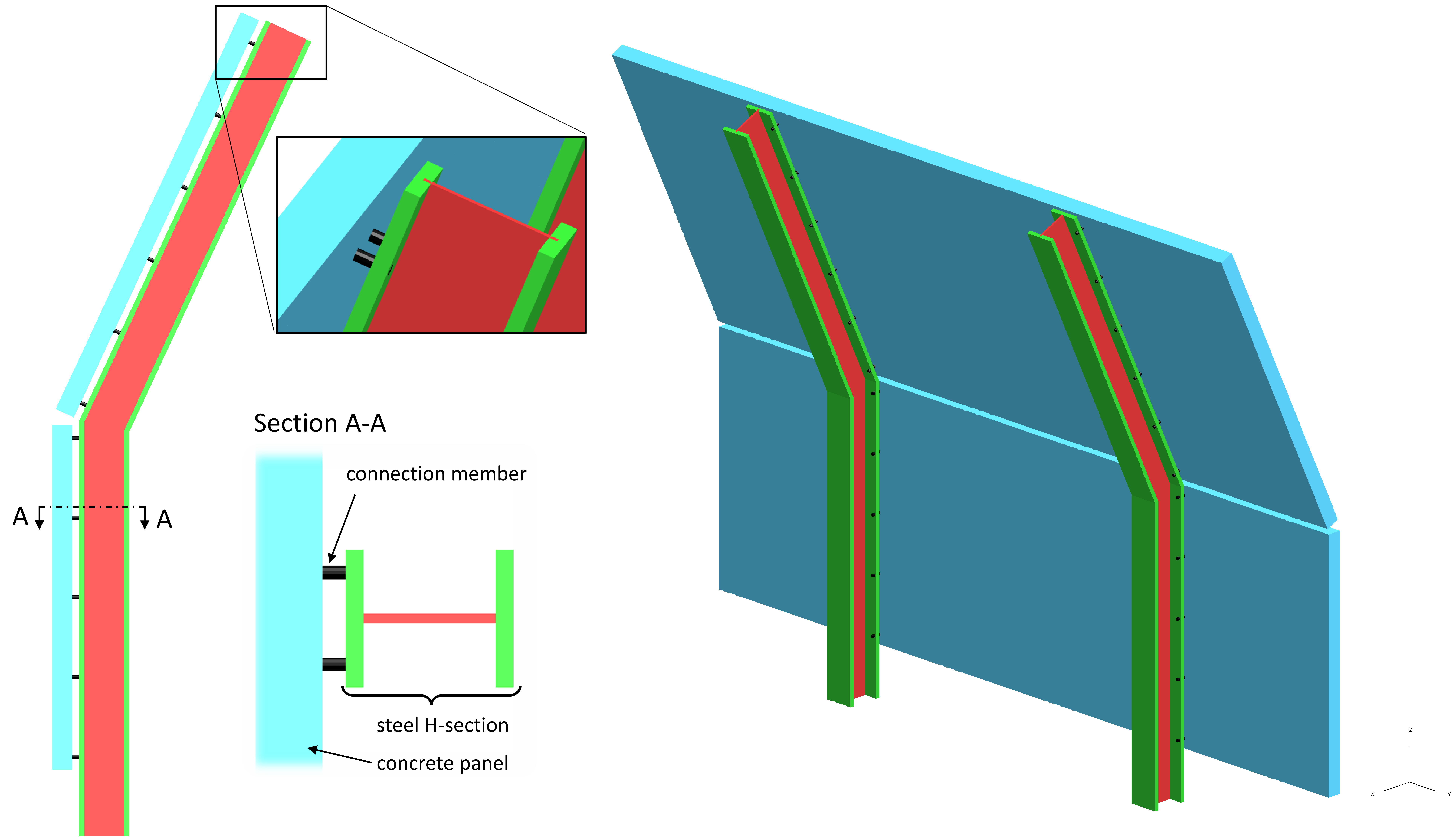
During the design of the cranked barrier, a number of early options were considered based upon a concept of steel H-posts and concrete panels attached to the outside as shown in Figure 12.
Various connections were considered at the “connection member” location shown in Figure 12 including:
- elastomeric washers to avoid stress concentrations;
- steel bolts under high preload;
- steel brackets.
It was difficult to design fatigue resistant connections considering the practicalities of construction tolerance and including the possible slip effects from thermal expansion.
Following constructability review and cost comparisons, a precast concrete panel system was chosen with a torsion beam connecting the panels to the piles and avoiding steel-to-concrete connections. The panels cantilever the full height of the barriers including the crank where needed.
Dynamic Analysis by Finite Element
Earlier it was concluded that analysis using the Tr + ic model was more time consuming than the Ril model owing to the need to vary k. The remainder of this paper therefore focusses on the Ril load model applied to FE models of the barriers.
The Noise Barrier FE Model
The cranked barrier was shown in Figure 1. For reasons covered below, the torsion beams were generally limited to a length of 6 m as indicated by the Finite Element (FE) model shown in Figure 13.
The dynamic analysis was completed using explicit time integration in LS-DYNA which is a nonlinear dynamic analysis package. The torsion beam was modelled with solid elements, and the concrete panel with shell elements. The piles were modelled with beam elements and springs were used to represent a range of bedding stiffness values.
The model was loaded by a moving pressure pulse across the surface of the elements at the speed of the train.
As the maximum line speed for the barrier is 320 kph (88.89 m/s) analysis was completed with the load model pressure pulse applied to the barrier at speeds from V = 88.89/1.3 = 68 m/s to V = 88.89 x 1.3 = 116 m/s in increments of 1 m/s. The speed range was considered to effectively include sensitivities to a change in structural frequencies and possible variations in the shape of the load model.
FE Results
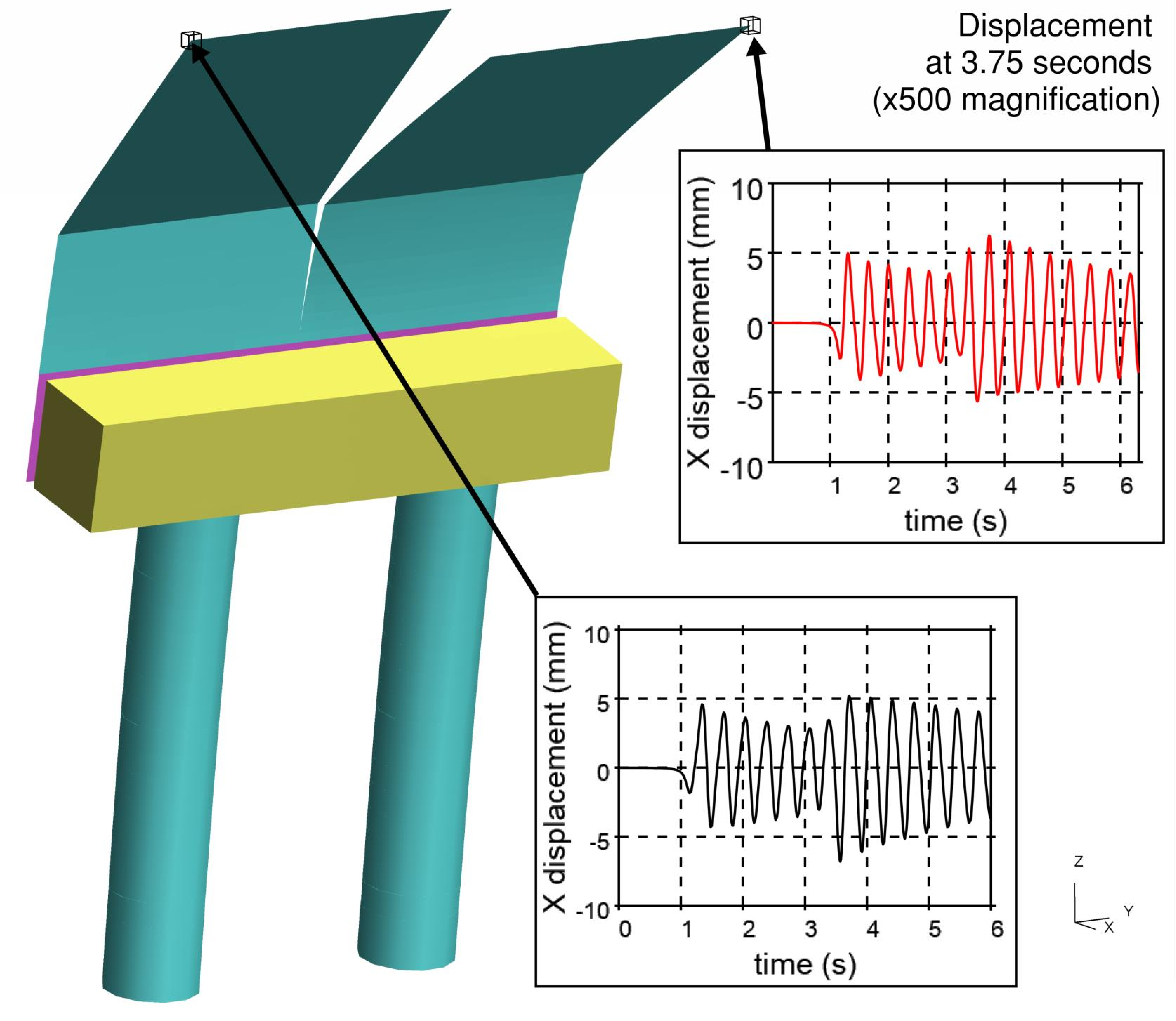
A plot showing the deformed shape of the noise barrier can be seen in Figure 14 for a train speed of 89 m/s. The plot also shows the displacement at the top of each precast panel which has a maximum amplitude of about 12 mm (-7 mm to + 5 mm).
The DAF values from the FE results were obtained by dividing the dynamic results by a pseudo static set of results obtained by passing the load model along the barrier slowly.
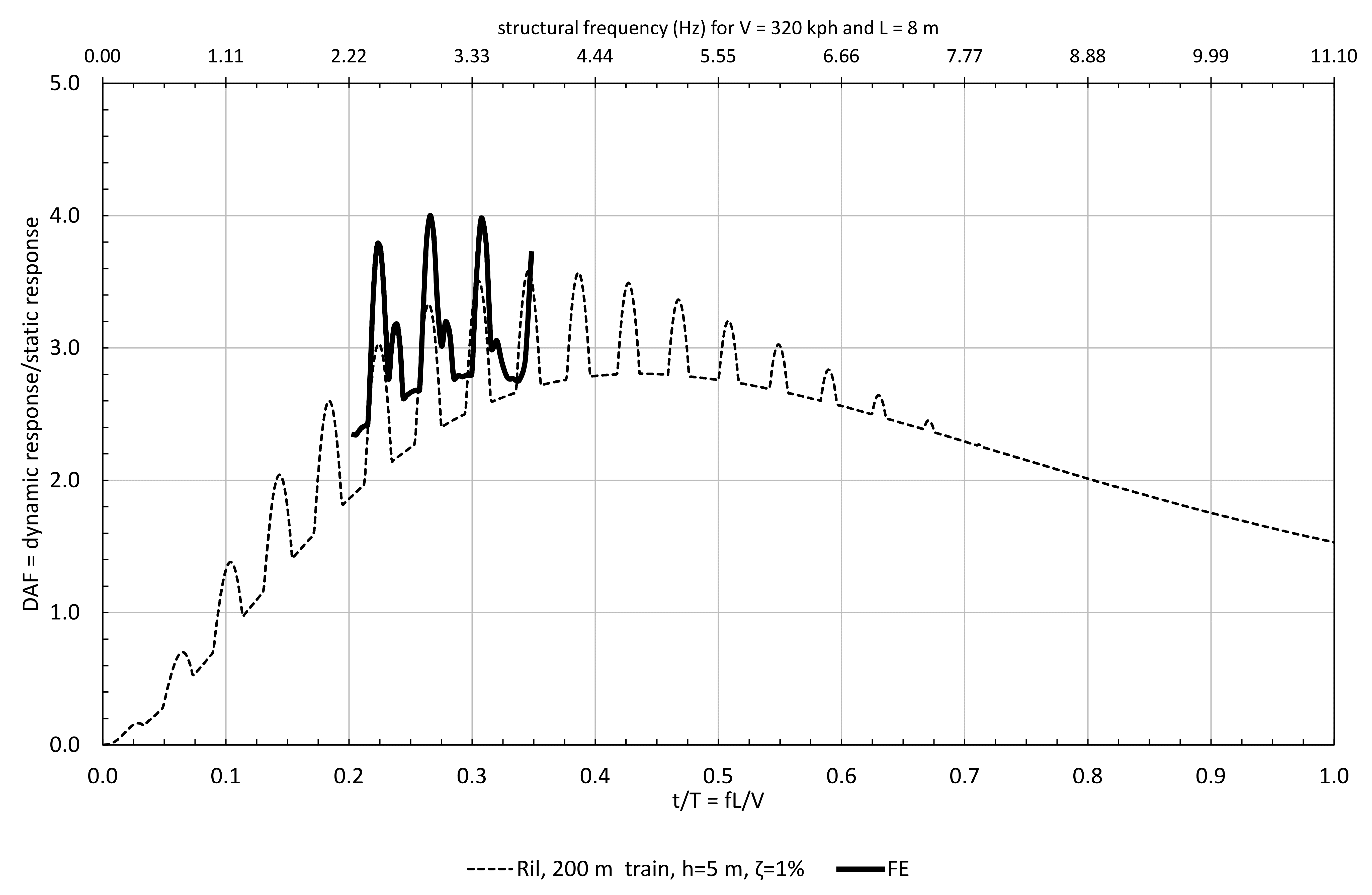
The resulting DAF values are plotted in Figure 15 for the Ril load mode and 1% damping (note that the first bending mode for this model was 2.96 Hz) along with the 1-dof values.
It can be seen that the two DAF plots are quite similar though the peak value for the FE model is slightly higher (4.0 v 3.6). This suggests that a preliminary design method using DAFs from a 1-dof system was reasonable in this case. However, this may not be the case in some circumstances as highlighted later in this paper.
Fatigue Results
As the design was for 6.88 million 200 m trains and 5.79 million 400 m trains over 120 years, it was determined early in the design process that fatigue would mostly govern the structure of the noise barriers.
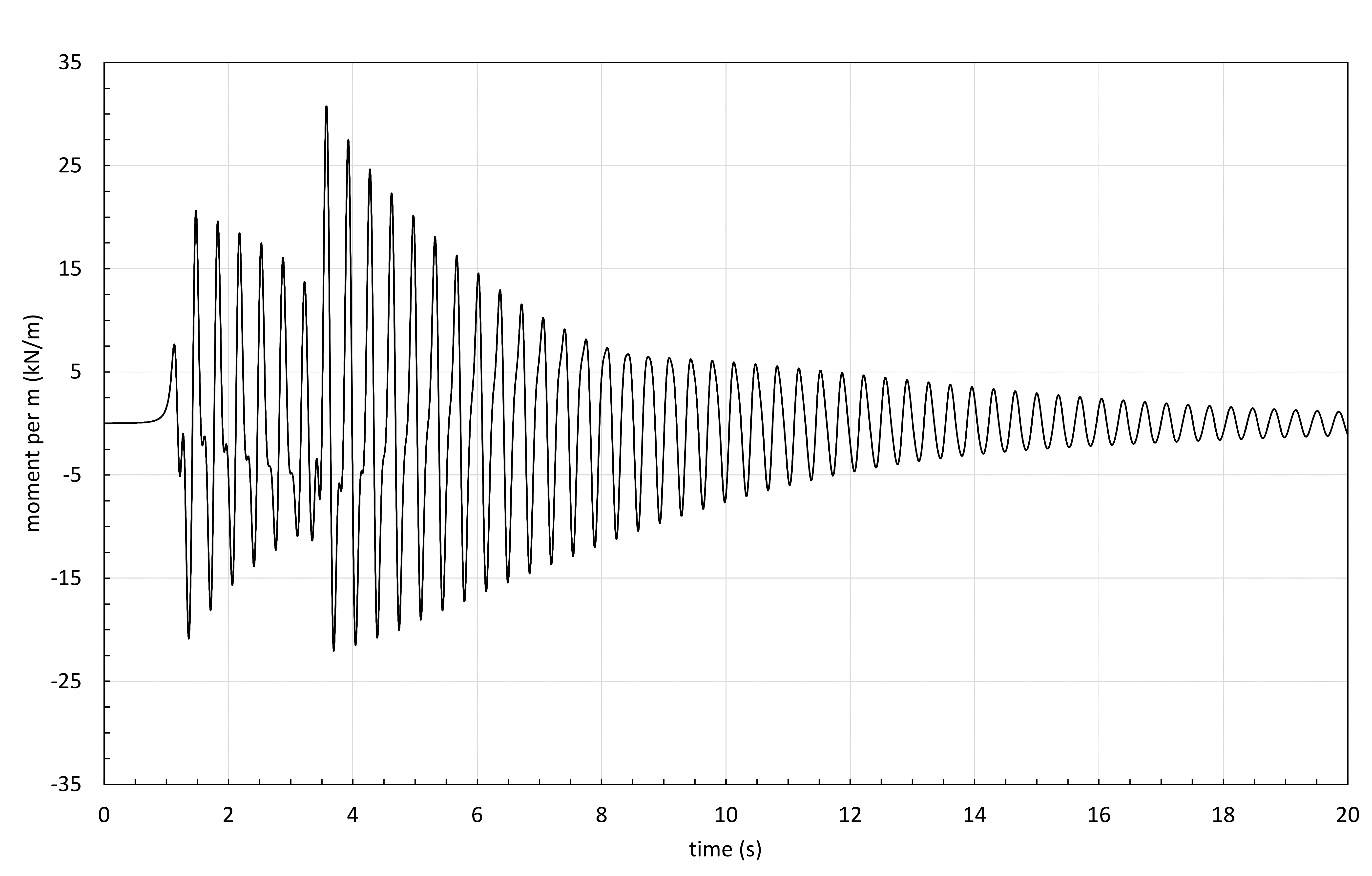
A typical plot of moment versus time is shown in Figure 16 for the response of the barrier with to the Ril 200 m train pulse (1% damping). This is plotted at the speed 89 m/s as this speed happened to be the most critical, which is why the large increase in vibration amplitude can be seen just before t=4 s, when the tail of the train arrives at the most additive time.
For unwelded reinforcing bar and more than 1 million cycles, it is noted that the damage is proportional to stress to the power of 9 [15]. With this in mind, the cycles in Figure 16 can be expressed as an equivalent number of cycles of the maximum amplitude. For example, the largest moment range is 53 kNm/m and the second largest of 48 kNm/m is equivalent to (48/53)9=0.41 cycles at 53 kNm/m. If this is repeated for all cycles in Figure 16, it can be determined that the cycles are equivalent to just over 2 cycles of 53 kNm/m. This observation is useful to quickly estimate damage prior to completing full fatigue calculations, particularly when combined with the DAF plots presented earlier along with static calculations.
For detailed design, the pulses were converted to stresses in the concrete and steel and rainflow-counting was undertaken to determine the cumulative damage.
End Effects on Longer Lengths of Noise Barrier
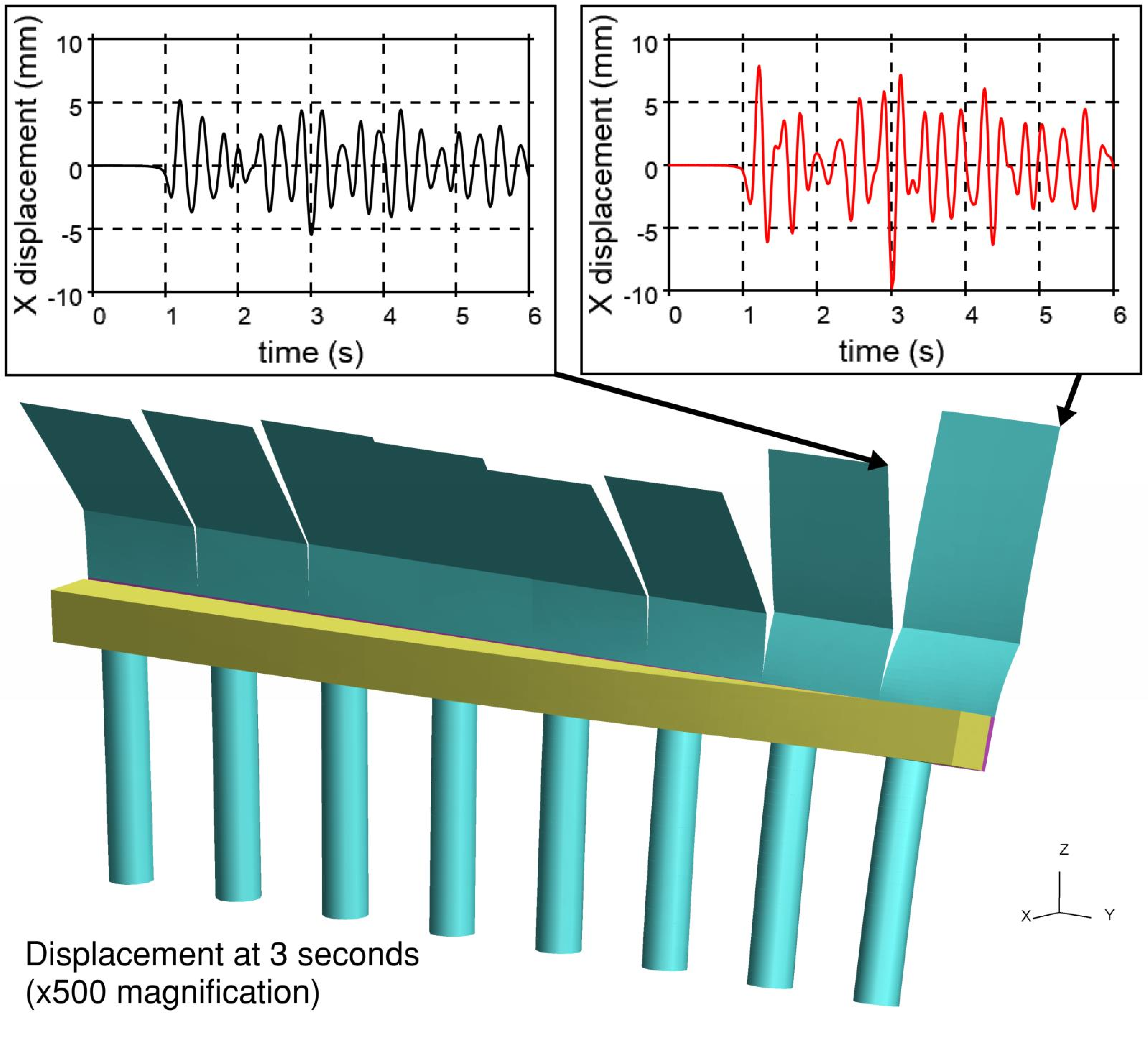
Originally a longer length of torsion beam was considered such as the 24 m long unit shown in Figure 17 which also shows the distortion amplitude up to 18 mm on the end precast panel versus only 10 mm on the interior panel.
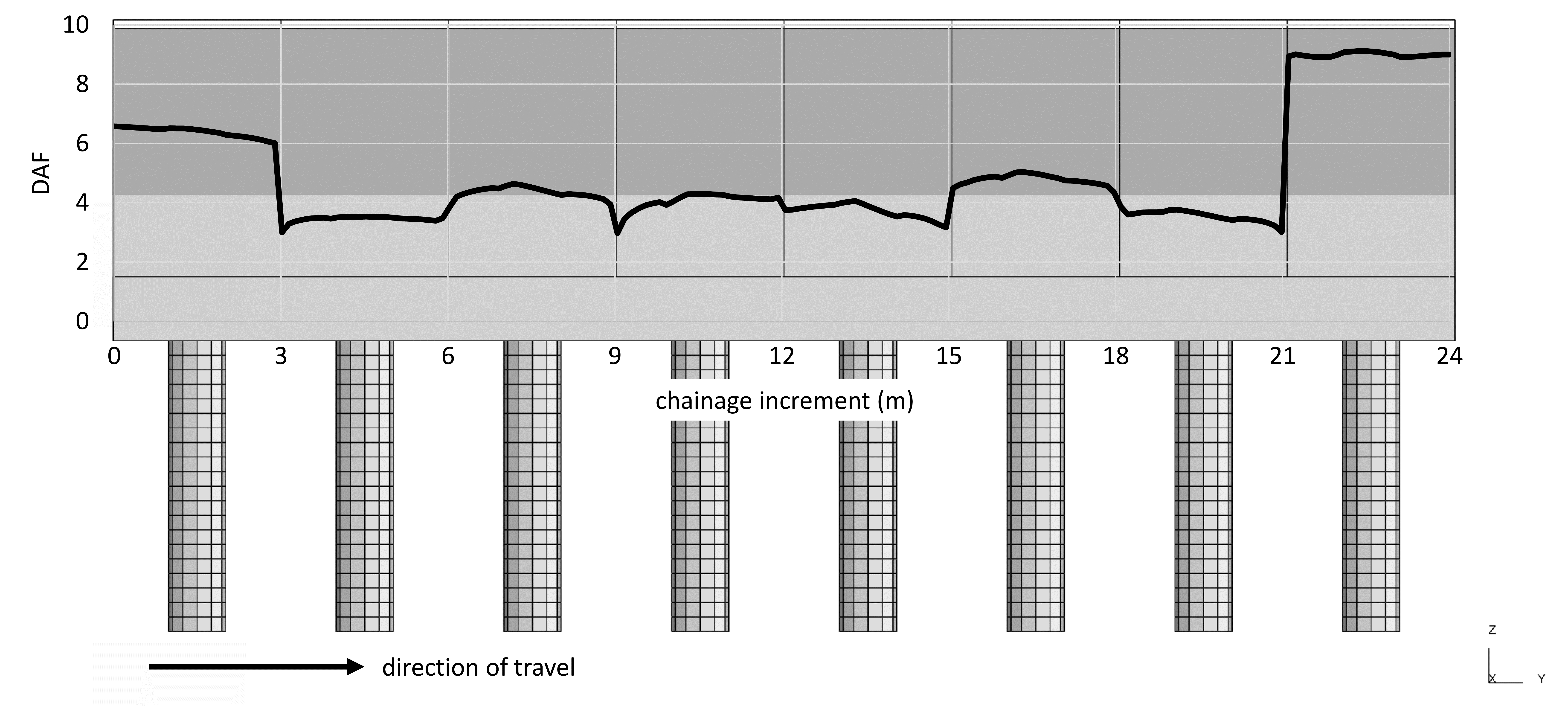
Figure 18 shows the DAF on the moment at the base of the barrier along the length at a train speed of 109 m/s (at this speed the DAF on the end panels was highest). A pseudo-static result was calculated by moving the pulse across the structure slowly (10 m/s), and the DAF was arrived at by dividing the dynamic peak values by the associated pseudo-static values.
It can be seen that there is a significant increase in DAF at the ends, reaching a value over 9 at the right-hand side. To design for this DAF would have required a significant increase in structural dimensions. Though not quantified, this effect was referred to by Hoffmeister[1].
The same DAF plot is shown in Figure 19 for the shorter 6 m long torsion beam which did not exhibit the same end effects. For this reason, the shorter length of torsion beam was adopted in the design. This also reduces thermal and shrinkage effects.
Testing
It is necessary to carry out cyclic fatigue testing of a noise barrier unit, and lateral cyclic loading tests of the piles, to verify the fatigue performance and damping. The purpose of the testing is to confirm the dynamic behaviour in a similar manner to the acoustic testing of the barriers as installed; it is not required as part of the design.
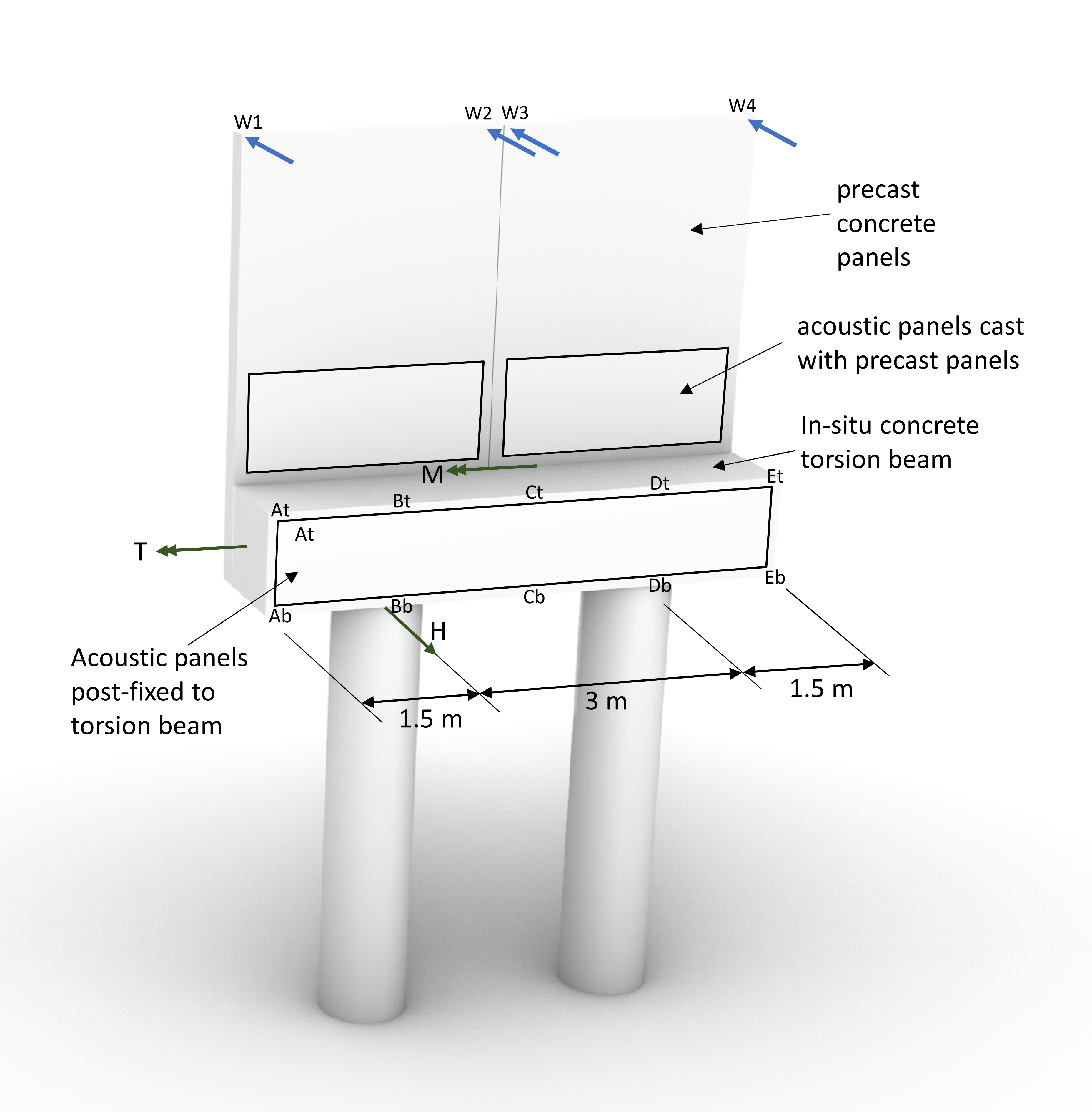
Figure 20 shows the proposed test layout with the inclusion of the acoustic absorber panels at the most highly stressed points.
Actuated point loads will be applied at locations W1 to W4 to achieve the target values of M, T and H (peak predicted fatigue values from the FE analysis presented earlier). Displacement will be recorded at locations A to E (10 points on torsion beam face) and W1 to W4. Additionally, strain measurements will be recorded on the reinforcing bar.
Conclusions
The dynamic fatigue design of the noise barriers at West Ruislip has been undertaken and the dynamics and fatigue aspects of this work have been presented.
The relevant European design codes have been reviewed along with published research on noise barriers.
The structural dynamic and fatigue design of high-speed noise barriers has been shown to be technically challenging and fatigue problems have been observed on other high-speed lines.
Limited load models have been found to be available for the design of noise barriers (compared, for example, to the number available for bridge design) and few results are published for full scale measured pressures on noise barriers. This paper therefore focussed on the load model in the German standard Ril 804.5501, along with a triangular load model proposed by HS2. Inferences were additionally drawn from published pressure measurements.
By considering these load models and showing the high dynamic factors and large number of resulting vibration cycles, it is not surprising that early noise barrier designs had fatigue problems. However, dynamic load models have recently been codified so these complex effects can be captured in the design.
The main highlights and conclusions of the paper are:
- Shock spectra have been developed for a proposed triangular load model and the load model in the Ril standard based upon the response of a 1-dof system.
- The Ril load model appeared to be easier to use as it had a broad spectrum and only a single pulse shape was able to generate a high dynamic response over a wide range of structural frequencies. The triangular model was considered but required several widths of triangle to avoid un-conservatism (relative to the Ril) at some frequencies.
- Inter-car pulses on the triangular load model were found to cause resonance at certain structural frequencies and this led to an increase in response of 23% for a noise barrier with 1% damping. However, it was noted that inter-car pulses in practice are more variable and would be unlikely to cause this level of response in barriers.
- The Ril pulse does not explicitly include inter-car pulses but it was considered by comparison to test results that it may have been scaled-up to implicitly include the effect.
- The FE results for the 6 m long cranked barrier unit at West Ruislip have been compared to the 1-dof shock spectra and were found to be in reasonable agreement for the short lengths of cantilever barrier considered.
- A continuous length of noise barrier has been found to have a significant dynamic amplification factor (DAF) at the beginning and end of the length. It was inferred that this phenomenon might also occur on some bridges. This should be considered in early design of bridges which are to be fitted with noise barriers. This effect is not indicated by a 1-dof system.
- Based upon the issues of end effects and high DAFs on cranked barriers, it seems clear that design requires dynamic finite element analysis to capture these issues.
References
[1] Hoffmeister B (2007) Development and Design of Noise Barriers for High Speed Railways, IABSE Symposium Report.
[2] Soper D, Gillmeier S, Baker C, Morgan T and Vojnovic L (2019) Aerodynamic forces on railway acoustic barriers, Journal of Wind Engineering and Industrial Aerodynamics 191, 266-278.
[3] BS EN 1991-2:2003 Eurocode 1: Actions on structures — Part 2: Traffic loads on bridges, BSI, London, UK.
[4] BS EN 16727-2-2:2016 Railway applications — Track — Noise barriers and related devices acting on airborne sound propagation — Non-acoustic performance Part 2-2: Mechanical performance under dynamic loadings caused by passing trains — Calculation method, BSI, London, UK.
[5] BS EN 14067‑4:2013+A1:2018 Railway applications – Aerodynamics. Part 4: Requirements and test procedures for aerodynamics on open track, BSI, London, UK.
[6] UIC Code 779-1 (2015) The effect of the slipstream of passing trains on structures adjacent to the track, second edition, January 2015.
[7] Deutsche Bahn AG, RIL 804.5501: Lärmschutzanlagen von Eisenbahnstrecken, 2007
[8] Lachinger S, Reiterer M and Kari H (2016) Comparison of calculation methods for aerodynamic impact on noise barriers along high speed rail lines, In: World Conference on Railway Research.
[9] Belloli M, Pizzigoni B, Ripamonti F and Rocchi D (2009) Fluid-structure interaction between trains and noise-reduction barriers: Numerical and experimental analysis, Numerical and experimental analysis. WIT Transactions on the Built Environment. 105. 49-60.
[10] Tokunaga M, Sogabe S, Goto K, Santo T, Tamai S and Ono K (2013) Dynamic response characteristics of the tall noise barrier on railway structures during passage of trains and its design method, Journal of Japan Society of Civil Engineers, Series A. 69. 392-409.
[11] Friedl H, Reiterer M and Kari H (2011) Aerodynamic excitation of noise barrier systems at high-speed rail lines – Fatigue analysis, IOMAC 2011 4th International Operational Modal Analysis Conference, Istanbul, Turkey.
[12] Baker C, Jordan S, Gilbert T, Quinn A, Sterling M, Johnson T and Lane J (2014) Transient aerodynamic pressures and forces on trackside and overhead structures due to passing trains. Part 1: Model-scale experiments, IMechE Journal of Rail and Rapid Transit.
[13] Harris C M and Crede C E (2002) Shock and Vibration Handbook, Fifth Edition, New York: McGraw-Hill, USA.
[14] Bathe K-J (1996, 2014) Finite Element Procedures, 1st Edition, Prentice Hall, 1996; 2nd Edition, 2014, Watertown, MA, USA.
[15] BS EN 1992-1-1:2004 + A1:2014 Eurocode 2 Design of Concrete Structures Part 1-1: General Rules and Rules for Buildings
Notation
f natural frequency of vibration
h height of point above top of rail
t pressure pulse normalised time duration
y horizontal distance from the track centreline to the barrier
z height of point above top of rail
![]() pressure coefficient
pressure coefficient
DAF dynamic amplification factor
H height of barrier above top of rail
L characteristic pulse length
P pressure
TOR top of rail
Tr + ic HS2 load model with inter-car pulses
Tr A hypothetical load model derived from the HS2 load model by removing inter-car pulses
V train speed
![]() air density safety factor (from Ril standard)
air density safety factor (from Ril standard)
![]() density of air
density of air
![]() damping ratio
damping ratio
Peer review
- Gennaro Sica, Senior Acoustics and Vibration EngineerHS2 Ltd