Predicting sound levels generated by jet fan ventilation systems in tunnels
The operation of jet fans to ventilate tunnels generates sound that propagates within the tunnels, and can be emitted to external locations, which may include noise-sensitive receptors. To achieve suitable predictions of noise impact, it is important to account for the propagation of sound inside tunnels, which is an engineering problem not addressed by current standards or codes of practice. A study was conducted to review existing approaches and determine a suitable model to predict tunnel sound propagation. Theoretical approaches were reviewed, and a 3D geometrical model was generated, the predictions of which were validated using empirical data. A simpler modelling approach identified from the literature was compared with the 3D model, and the differences observed were analysed. The study concludes that the simple model could be used to obtain reasonably accurate estimations, which can be made conservative by applying adjustments to the predicted sound levels.


Introduction
The tunnel ventilation system design proposed for High Speed Two (HS2) incorporates jet fans (which are commonly used in road and railway tunnels), to provide ventilation and temperature management in the event of emergencies, and if railway congestion occurs, causing trains to queue in tunnels.
The potential for sound from jet fan operation to propagate to noise-sensitive receptors outside the tunnels can be estimated using indicative source information alongside appropriate prediction methods. However, there is a lack of standardised and validated approaches to predicting sound propagation in such environments as tunnels, which do not conform to the assumptions inherent in the most simplistic engineering expressions for reverberant sound fields. Furthermore, as will be shown below, the influence of directional characteristics of a real source such as a jet fan will affect the propagation of sound within a tunnel. This behaviour limits the applicability of existing tunnel sound prediction models, which have typically been developed for predicting the sound from road vehicles inside tunnels.
This paper describes approaches to addressing this engineering problem: firstly the relevant characteristics of jet fans are described with reference to empirical data; secondly, some aspects of ‘long room’ acoustics are reviewed, highlighting some of the challenges in accurate sound propagation modelling for such an environment. A dataset of tunnel sound propagation measurements, captured during the development of the design for a previous railway project, is described and used as a validation reference. Tunnel sound propagation prediction models identified in the literature are examined and used alongside a 3D geometrical model to make estimations of sound propagation, which are compared with the validation data. The validation results, and the advantages or disadvantages of each approach are discussed, and the expected interaction effect of jet fan source characteristics with the tunnel models is also considered. The 3D model is then used to develop adjustment terms for a more simplistic modelling approach, in order to make estimations of jet fan source-specific sound propagation in tunnels that are expected to be slightly conservative.
Previous studies concerning jet fan sound in tunnels have been conducted by Ridley et al[1] and Richardson et al[2]. Ridley et al compared an implementation of a geometrical acoustics model developed by Kang[3] with measurements of broadband noise made in a rectangular road tunnel up to a range of 120m; the results indicated reasonable agreement at lower frequencies[1]. Richardson et al used a commercial geometrical acoustics software tool (Odeon, discussed further below) to predict jet fan sound propagating within a road tunnel and a separate noise mapping tool to predict sound immission levels at receptors; an identical exercise to the motivation behind the present study. No validation exercise was reported in the publication, and no consideration of the effect of jet fan directivity is evident[2].
Jet fan sound
Jet fans are typically used in tunnels and car parks for ventilation and rapid dispersion of fumes or smoke. They normally comprise an axial flow fan inside a cylindrical housing, and are designed for efficient, high-thrust performance. The fan and high-thrust ‘jet’ generate relatively high sound levels, and jet fans are usually installed with sound attenuators fitted.
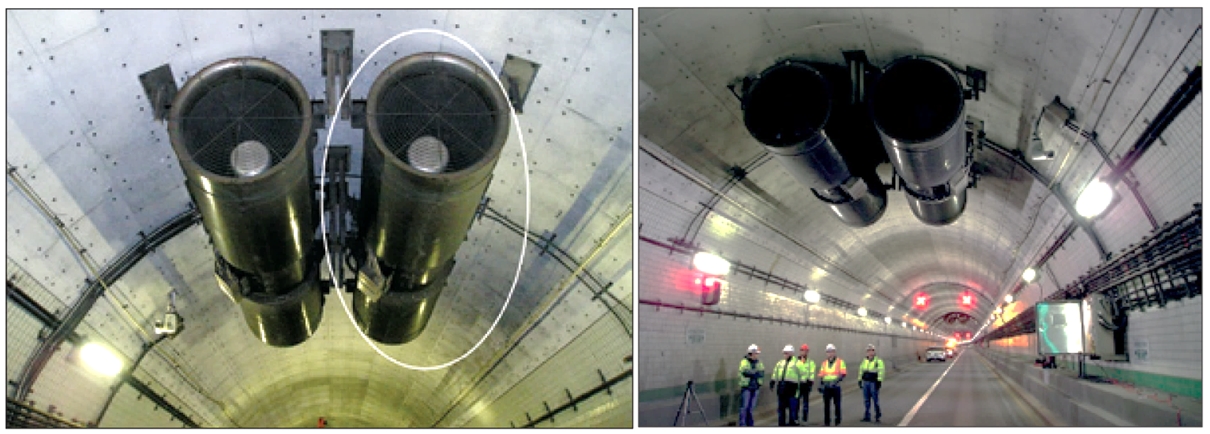
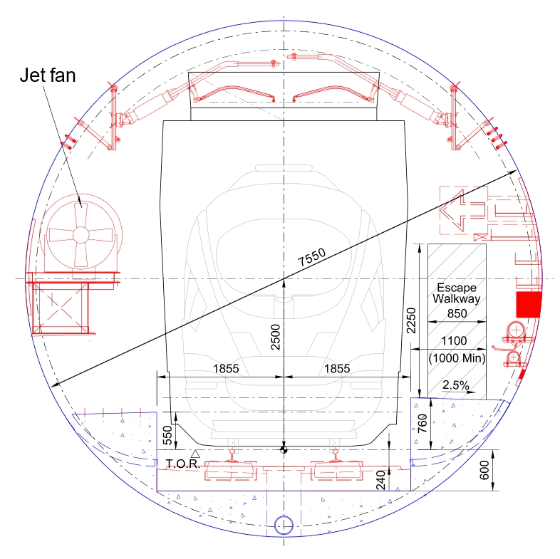
As illustrated in Figure 1, tunnel jet fans comprise relatively large assemblies, eg ≥1 m in diameter and several metres in length. The primary sound source radiation points would be at each of the open ends of the cylinder, although the casing itself will also radiate some sound. In this study, jet fans have been modelled as a single (directional) point source, as only the sound propagating towards the end of the tunnel is of interest here. If a more accurate characterisation of the sound field near to the jet fan were needed, it would be necessary to consider the spatial distribution and physical nature of the source emission points in greater detail.
Some jet fan designs allow reversible operation, ie the direction of flow can be switched. This reversibility will generally result in different sound attenuation performance in each direction due to the effects of dynamic flow on the attenuator insertion loss. Since a jet fan is effectively a sound pressure source placed inside a long tube, jet fans also exhibit a directional sound radiation characteristic[4], which will affect the way in which the sound propagates along a tunnel. This is an important aspect of the problem that has been investigated in this study.
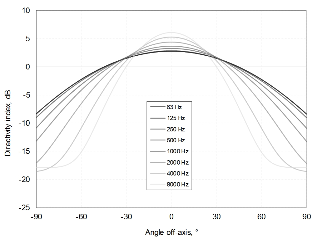
Jet fan sound measurement data from the study reported by Thalheimer et al[4] have been used to estimate the directivity characteristic. The measurements were acquired during testing conducted at a supplier facility and were limited to directions of 0° and ±45° (relative to the axis normal to the jet fan opening). The test facility comprised a partially open building and some influence of reflection and diffraction from solid surfaces on the measurements cannot be ruled out; nonetheless, the data are considered indicative, and the background ambient time-averaged sound levels (Leq,T) were more than 10 dB below the jet fan sound levels in all octave bands. The measured sound pressure levels have been used to derive estimated directivity indexes via a least-squares (2nd order) regression over the emission angles, and subtraction of the resulting spatial average sound pressure from the directional value at each angle. The resulting directivity indexes (DIs) have then been adjusted according to the practical ‘atmospheric scattering bound’ limit estimation equation advised by Bies et al[5], after Davy[6], ie:

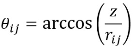
Where DI and DIb are (respectively) the unbounded and bounded directivity indexes at emission angle ![]() , and
, and ![]() is the maximum positive directivity index – these values are all determined at separate frequencies, octave bands in this case. The estimated octave-band directivity values derived using this process are shown in Figure 2.
is the maximum positive directivity index – these values are all determined at separate frequencies, octave bands in this case. The estimated octave-band directivity values derived using this process are shown in Figure 2.
Long room acoustics
Simplistic engineering descriptions of the acoustical environment in an enclosed space usually make the assumption that the sound field is diffuse (ie all possible wave directions are equally probable and waves interact with effectively random phase relationships such that the energy is summed incoherently), and that the time-averaged reverberant field is uniform (ie spatially invariant). These conditions are never exactly achieved in reality, although they are approached to a sufficient degree in some spaces that the expected steady-state airborne sound field generated by a single, theoretical point source can be approximated using the following simple expression[5], the two separate terms in which describe the direct and reverberant components of the total field:
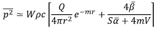
Where ![]() is the mean-square sound pressure, W the acoustic power,
is the mean-square sound pressure, W the acoustic power, ![]() the air density, c is the sound speed in air, Q is the source directivity factor, is the direct distance from the source to the receiver, S is the total surface area within the space, V is the free volume, m is the energy propagation coefficient in air,
the air density, c is the sound speed in air, Q is the source directivity factor, is the direct distance from the source to the receiver, S is the total surface area within the space, V is the free volume, m is the energy propagation coefficient in air, ![]() is the (locally-reacting) surface mean intensity absorption coefficient, and
is the (locally-reacting) surface mean intensity absorption coefficient, and ![]() the corresponding mean reflection coefficient. In addition to the diffuse-field assumption, Equation 2 implicitly assumes that the calculation point is in the far-field of the source, so that all sound field components are composed of effectively-plane waves. The e-mr and 4mV terms representing sound energy dissipation via viscous losses in air are often neglected in small and medium-sized rooms, or if only lower frequencies are important. As is shown below, for long range propagation within large tunnels, air absorption should be accounted for.
the corresponding mean reflection coefficient. In addition to the diffuse-field assumption, Equation 2 implicitly assumes that the calculation point is in the far-field of the source, so that all sound field components are composed of effectively-plane waves. The e-mr and 4mV terms representing sound energy dissipation via viscous losses in air are often neglected in small and medium-sized rooms, or if only lower frequencies are important. As is shown below, for long range propagation within large tunnels, air absorption should be accounted for.
The practical applicability of Equation 2 is limited to the sound field region with high modal density in rooms of simple, cube-like forms, containing a fairly uniform spatial distribution of surface absorption properties, which comprise relatively high reflectivity[7]. These types of enclosures are commonly referred to as ‘Sabine’ spaces, as Sabine’s statistical reverberation theory[8] (and related theories) can be supported only in a well-diffused field. Equation 2 will fail to accurately describe the sound propagation in a tunnel or ‘long room’, with one dimension out of proportion to the others. In such spaces, the diffuse-field assumptions cannot hold, and both the reverberant and direct field components decay with distance from the source[9].
To avoid misapplication of purely statistical theories based on the diffuse field assumption, a geometrical acoustics approach can be taken to estimate the expected sound field in a long room (a recent review of geometrical acoustics is given by Savioja et al[10]).. This approach treats the propagation of sound waves in terms of ‘rays’, which are vectors that define the predicted path of a wave in any given direction. The ‘method of images’, (or ‘image source method’, ISM) is one such geometrical approach, which has its origins in the work of Leonhard Euler[11]. Applications of the ISM to tunnels are discussed further below, but an ISM study often cited in the acoustics literature is that of Allen and Berkley[12], which exemplified the method with FORTRAN code.
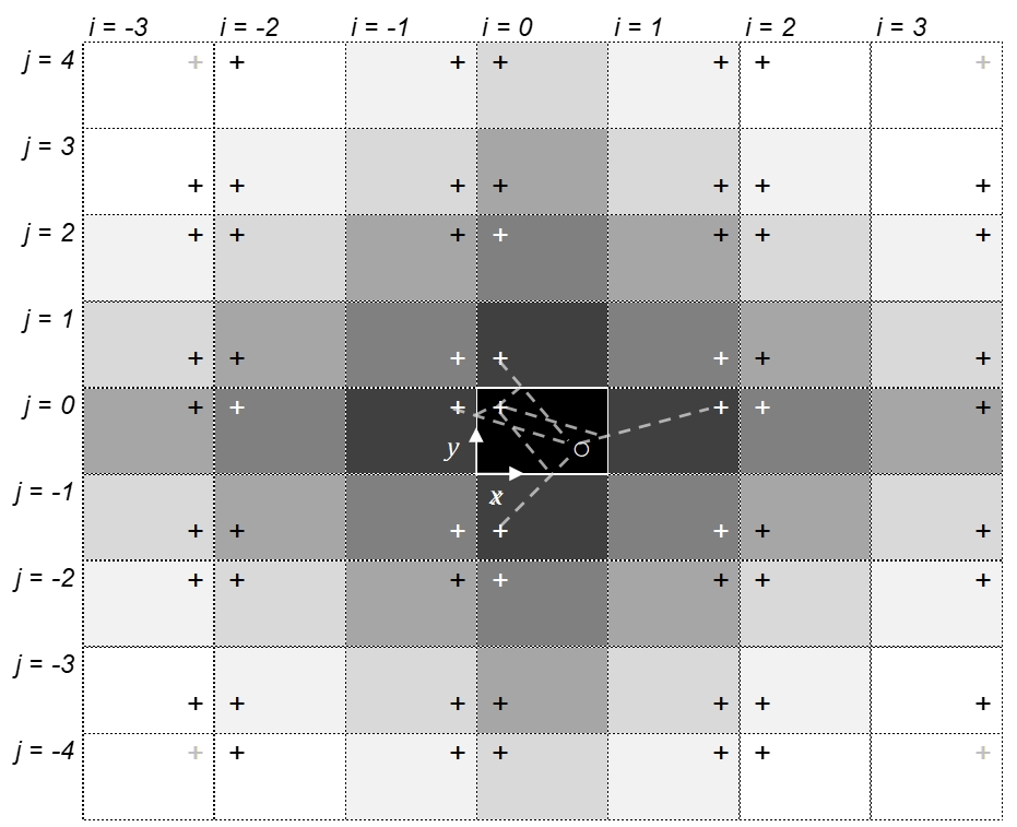
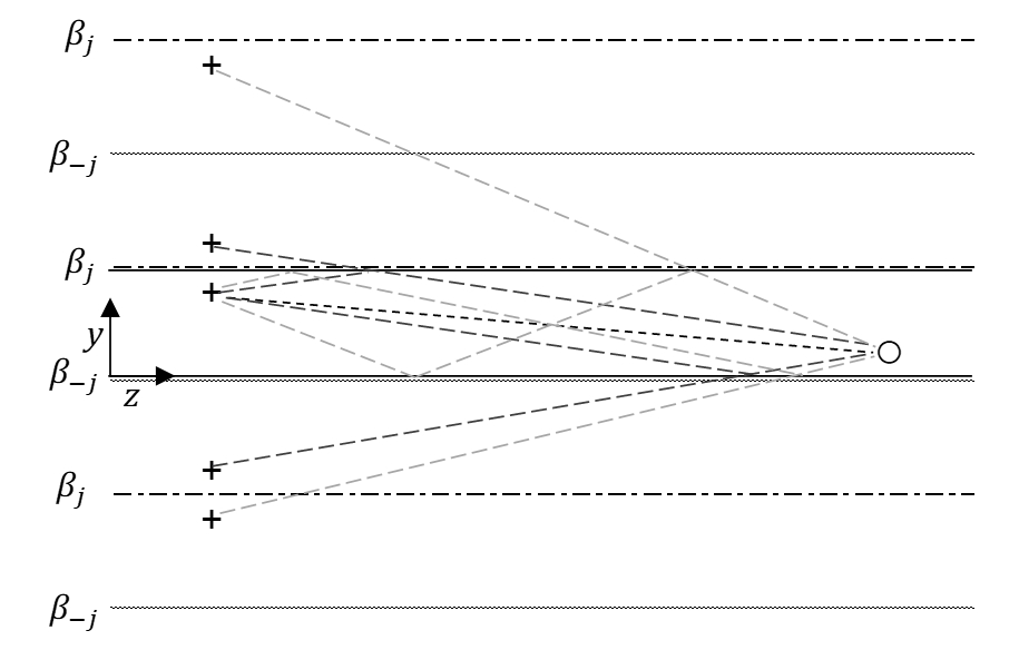
The ISM characterises enclosed sound fields by replacing each surface-reflected sound ray with a direct ray path from an equivalent ‘image source’, situated in a virtual ‘image domain’ beyond the real enclosure boundaries. The ISM concept is illustrated in Figure 3, which shows part of an ‘image plane’ for an infinitely long rectangular room, the long dimension of which extends along the axis normal to the plane. The real source (‘+’) and receiver (‘o’) appear situated in the central box (which represents a cross-section through the long room), and are separated by some distance along the long dimension (z-axis). The direct paths from each image (‘+’, shaded boxes) to the receiver represent i, j orders of reflection from the real room surfaces – first-order reflected paths are indicated in Figure 3 by dashed lines.
The ISM has some disadvantages, in particular with more-complicated geometries and multiple reflections, which entail exponentially increasing numbers of images to be included in the calculation– this leads to high computational expense[13], although methods to mitigate this drawback exist[14]. It also must be combined with other methods (such as ray-radiosity) if diffuse, rather than specular, reflections are to be modelled to represent surface scattering. However, for low-absorption, effectively rigid, smooth surfaces and simple geometries, its accuracy approaches exact solutions to the wave equation[15]. Furthermore, it is particularly well-suited to tunnel applications, as the computational expense is limited by the lack of end surfaces and the associated omission of one entire dimension of image sources – for an enclosed room the image domain would be three-dimensional, rather than planar. On the other hand, the circular geometry of a curved tunnel may be too complex to explicitly model using ISMs. However, as will be shown, close representation of curved geometries using the ISM is not always necessary to achieve acceptably accurate predictions.
The ISM geometrical approach can be used to simulate complex pressure fields (as rays), which can model the effects caused by wave interference[14]. However, since it cannot model diffraction or diffuse reflection, in general, the ISM remains an approximation to full-wave solutions[16]. Most commonly, it is applied in conventional practice and commercial software tools as a sound energy propagation model, which disregards the complex pressure phase. However, ‘wave-based geometrical acoustics’ software tools implementing the ISM have also been developed, which allow wave interferences and modal resonances to be included[17].
In enclosed spaces, modal resonances caused by wave interference occur at frequencies dependent on the geometry of the free air volume (as well as the surface impedance properties). The modal responses of enclosures are increasingly important with decreasing frequency, as the density of mode frequencies reduces, and resonances become decisive in determining the response. Provided its cross-sectional dimensions are sufficiently large compared with all wavelengths of interest to allow sound energy to radiate freely from ends (without inertially-reactive reflections), a tunnel can be thought of as a type of waveguide of effectively infinite length. In this case only cross-modes (ie transverse and radial modes and modal combinations) are of importance, as the existence of longitudinal modes is prevented. The cross-mode frequencies f m,n for a rigid cylinder can be calculated using[18][19]:
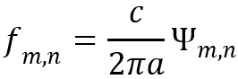
Where m, n represent the transverse and radial modal orders respectively (ie the number of pressure nodes in the corresponding eigenfunctions) a is the cylindrical radius, and ![]() represents the nth root of the derivative of the mth-order cylindrical Bessel function of the first kind, J’m. The mode frequencies can be used to determine the modal density, which indicates the spectral regions within which resonant modal responses are likely to be of importance in determining the sound field behaviour, and vice versa. For calculations in relatively wide frequency bands, such as octave bands, it has been suggested that a modal density of around three or more (ie at least three mode frequencies present within the band), indicates the start of the region of the spectrum in which modal behaviour may be neglected[5].
represents the nth root of the derivative of the mth-order cylindrical Bessel function of the first kind, J’m. The mode frequencies can be used to determine the modal density, which indicates the spectral regions within which resonant modal responses are likely to be of importance in determining the sound field behaviour, and vice versa. For calculations in relatively wide frequency bands, such as octave bands, it has been suggested that a modal density of around three or more (ie at least three mode frequencies present within the band), indicates the start of the region of the spectrum in which modal behaviour may be neglected[5].
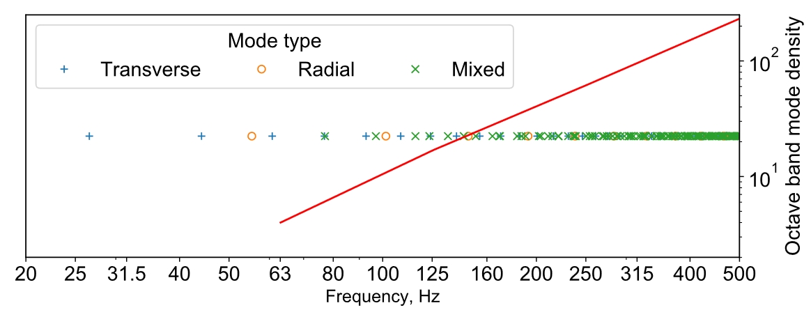
As shown in Figure 4, Equation 3 has been used to calculate the cross-mode frequencies and octave-band modal densities up to 500 Hz for a rigid cylinder of diameter 7.55m (which represents the size of the railway tunnels considered in this study). Figure 4 shows that the derived mode densities follow a logarithmic profile, increasing quickly from a value of 4 in the 63 Hz band. While the real railway tunnels considered here are neither perfectly cylindrical nor rigid, this result, alongside the knowledge that jet fans generate sound over a broad frequency range, is an indication that the enclosure modal response may not be of importance within the context of estimating octave-band sound propagation from jet fans in tunnels. As will be shown below, this indication is also supported by modelling results for a railway tunnel with similar dimensions.
Tunnel sound propagation measurements
To ensure the application of a suitable prediction model, validation exercises have been undertaken using relevant measurement data. A suitable measurement dataset was collected during a test intended to simulate a jet fan installation in a railway tunnel. A hemi-dodecahedron loudspeaker suspended 2.5 m above the access walkway, was used to emit broadband sound along the tunnel (approx. 7.6 m diameter), with a frequency spectrum shaped to match that of a candidate jet fan system. The reported source sound power (Lw) spectrum is shown in Table 1[20].
| Octave band frequency, Hz | 63 | 125 | 250 | 500 | 1000 | 2000 | 4000 | 8000 | dB(A) |
|---|---|---|---|---|---|---|---|---|---|
|
Lw, |
103 |
103 |
105 |
97 |
97 |
94 |
90 |
86 |
102 |
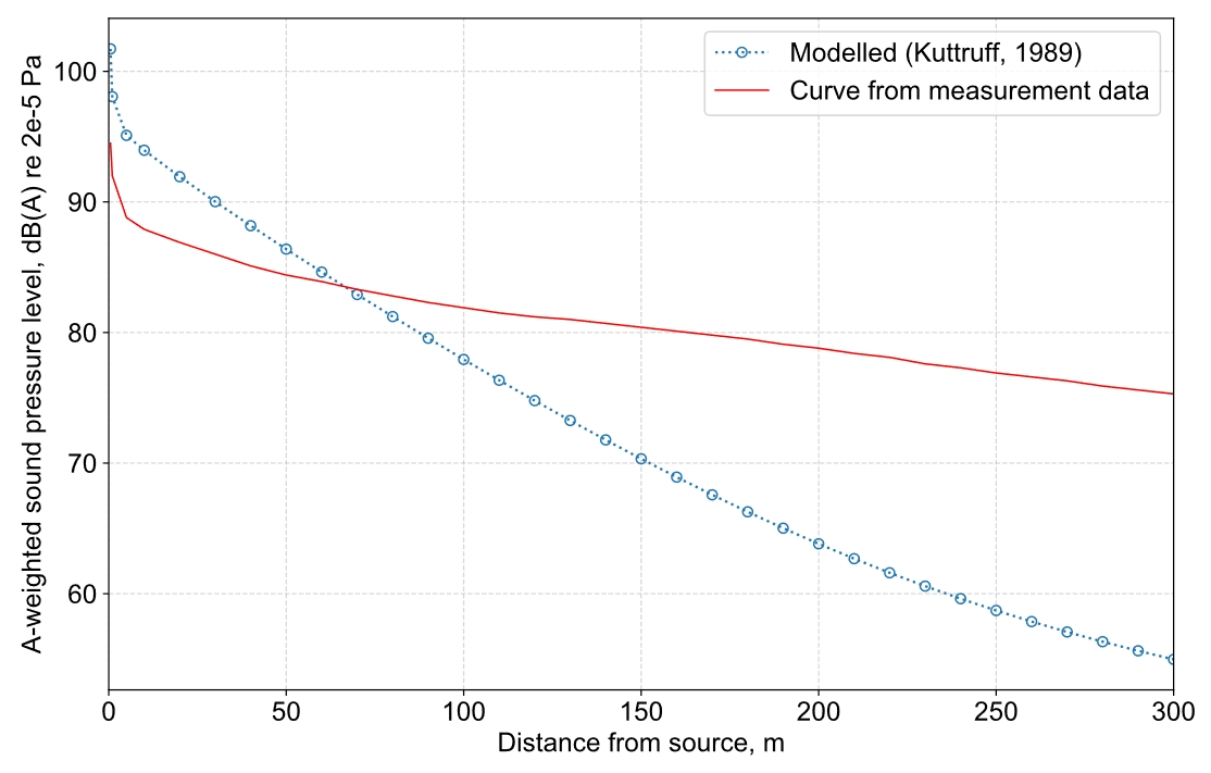
The measurement results are shown in Figure 5[20], which presents the individual measurements alongside a fit curve, as originally reported (NB, the fit curve was not reported as being derived using a statistical model; it appears to have been manually traced through the data). The measurements reported comprise overall A-weighted levels only; spectral data are not included.
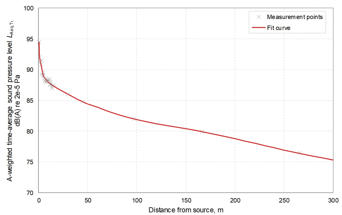
Figure 5 shows that, beyond ~100m, the attenuation of the A-weighted level settles into a linear relationship with distance, reducing at a rate of ~3.3 dB per 100m.
The type of speaker used in the test described above is designed to have negligible source directivity over its radiating hemisphere, whereas a real jet fan is expected to exhibit significant directivity, as discussed above.
Tunnel sound propagation modelling
Models of long room (and tunnel) sound propagation identified in the literature can be separated into those based on the coherent (pressure-based) and incoherent (energy-based) ISMs, numerical wave-based methods, and others, such as semi-analytical methods; some of the published approaches identified in this study have previously been reviewed by Kang[9].
Model inputs
A diagram of the cross-sectional geometry considered in the calculations made using the models discussed below is illustrated in Figure 6, which shows a 7.55m Ø tunnel with a typical jet fan installation at one side.
The sound absorption of tunnel surfaces has been assumed to be represented by the values shown in Table 2. While real tunnels will include cables and equipment, it is assumed that these will have a negligible effect on the total sound absorption. The open tunnel ends are assumed to be 100% absorptive at all frequencies.
| Octave band frequency, Hz | 63 | 125 | 250 | 500 | 1000 | 2000 | 4000 | 8000 |
|---|---|---|---|---|---|---|---|---|
|
Coefficient |
0.02 |
0.02 |
0.03 |
0.03 |
0.03 |
0.04 |
0.07 |
0.07 |
The effects of air absorption have been modelled where relevant using frequency-dependent attenuation coefficients calculated according to ISO 9613-1:1993 [22], using central parametric assumptions of 20°C temperature, 70% relative humidity, and 101.325 Pa atmospheric pressure. The speed of sound in air at 20°C is taken to be 343.3 ms-1.
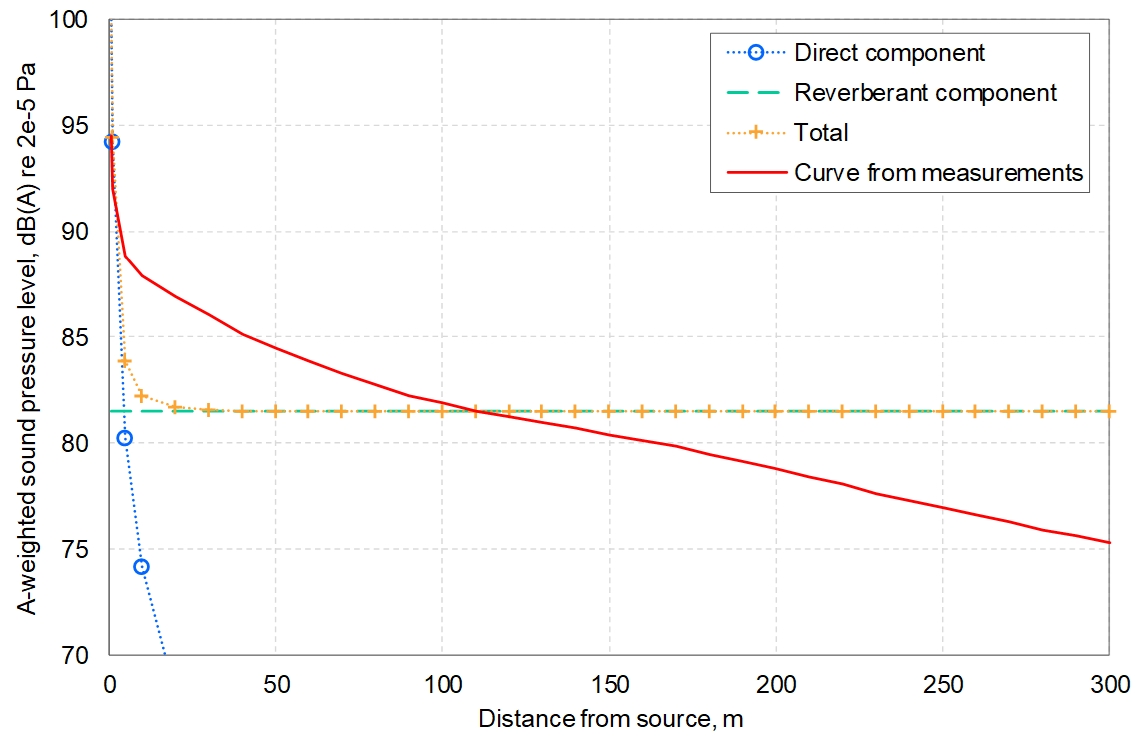
The diffuse-field model defined in Equation 2 has been used to calculate a sound level as might be expected according to the assumptions of this approach, as shown in Figure 7 alongside the measurement data. Figure 7 demonstrates the inadequacy of the diffuse-field assumption in describing tunnel sound propagation, showing that levels are greatly underestimated at shorter ranges and overestimated at longer ranges, with error magnitudes in the overall A-weighted levels reaching ±6 dB.
Incoherent image source method
Two types of incoherent ISM are discussed here: the first is the ‘full’ ISM, such as the models described by Gibbs et al[23], Galaitsis et al[24], and Kang[3]; the second comprises statistical simplifications of the full method, such as that represented by the model developed by the Acoustical Society of Japan (ASJ)[25][26][27][28][29][30][31]. In either case, by summing the source energy incoherently, phase interference effects are disregarded, as are phase changes at reflections.
BBN Model
The full ISM model presented by Galaitsis et al[24] was developed by Bolt Beranek and Newman (BBN) consulting engineers for predicting sound levels inside rectangular mining tunnels. The BBN model has been found to be more useful for the present application than Kang’s[3] model, which is limited to calculating relative sound levels and to receiver points along the geometric centre of the tunnel, whereas the BBN model predicts absolute levels (the main quantity of interest in this study), and is flexible regarding receiver placement.
The BBN model can be expressed as follows:
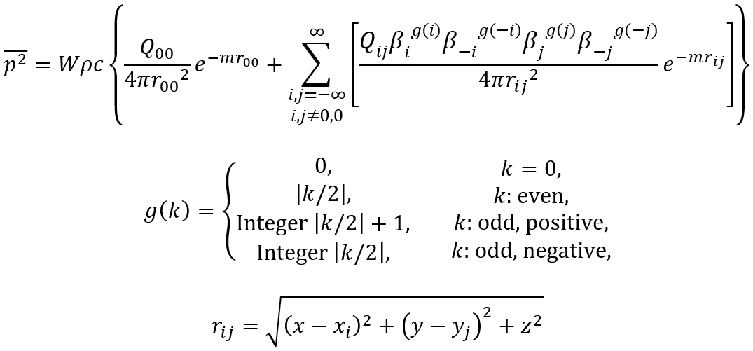
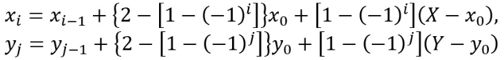
Where i, j are the indexes of each image source as indicated in Figure 3, and the βk terms represent the intensity reflection coefficients for each of the four tunnel surfaces in the direction of the indicated index. As illustrated in Figure 8, the reflection coefficients alternate recursively for each ‘image tunnel’ along both of the ‘short’ (x, y) dimensions. The source is located at (x0, y0, 0) and the receiver point is located at (x, y, z); the location of the (i, j)th image source (ie at zij = 0) is determined using:
where X and Y are the tunnel dimensions along the x and y axes, respectively.
The BBN model described by Galaitsis et al[24] has been augmented in Equation 4 by introducing two additional features not present in the original formulation: air absorption (represented by the e-mr terms) and source directivity (represented by the Q terms). The source (and image source) directivity terms are functions of the emission angle θ (for simplicity it is assumed that the source directivity is rotationally symmetrical around the z-direction), which is obtained from:
The augmented BBN model has been implemented in a Python program and used to calculate the expected sound propagation along the validation test tunnel. The calculation was based on assigning the tunnel 7.55m Ø directly to the rectangular dimensions used in the model. A convergence test on the BBN model calculations was conducted to determine an appropriate number of images to include, using steps at 2.6k (ie i, j = ±25), 10.2k (ie i, j = ±50), 40.4k (ie i, j = ±100), 90.6k (ie i, j = ±150), and 160.8k (ie i, j = ±200). In this case, the calculations exhibited convergence by 40.4k images; the other BBN model calculations discussed in this section were therefore obtained using this input value.
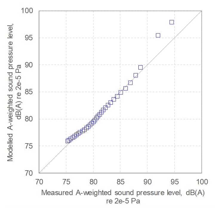
The results of the BBN model validation are shown in Figure 9 and Figure 10. It can be seen that the predictions including the effects of air absorption closely follow the measured levels, with error <1 dB for distances of ≥5m (root-mean-square error over this distance range is 0.4 dB); within 5m, errors are ~3 dB, with a systematic over-estimation observed. These error values are consistent with the original validation results presented by Galaitsis et al[24].
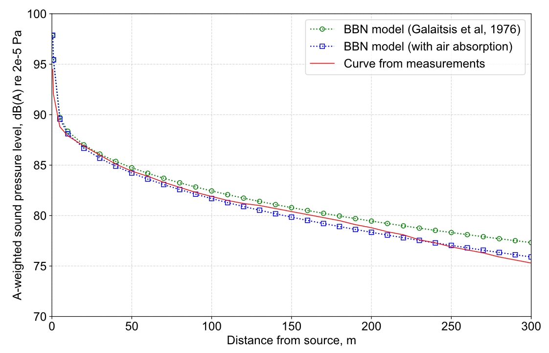
Also shown in Figure 9 are the predictions using the original BBN model, ie excluding air absorption – it can be seen that this results in slightly higher levels, which appear to diverge with increasing distance. It is acknowledged that this observed effect could also be partially explained by differences in surface absorption properties (eg the assumed surface absorption may be lesser than actually present in the tunnel), however, since air absorption would inevitably have affected the test measurements, this indicates that the selected surface absorption coefficients in Table 2 are appropriate, and that the extension of the BBN model to include air absorption yields more accurate predictions – it is notable that the calculations in [24] are for distances <100m, so the air absorption effect may have been negligible for the sizes of tunnels considered by Galaitsis et al.
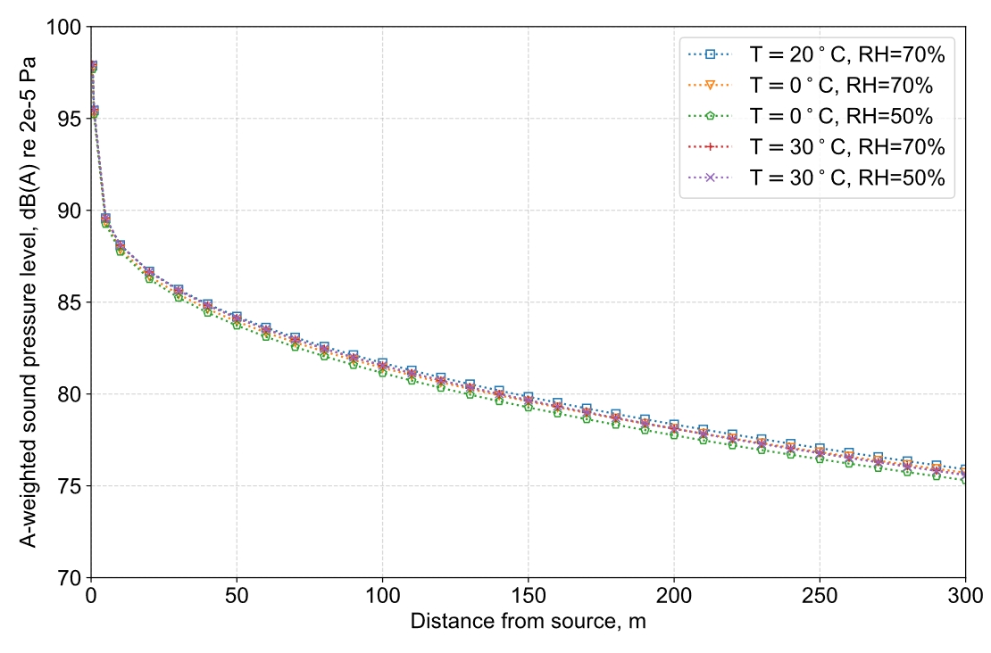
Air absorption is influenced by the temperature, humidity and atmospheric pressure, so a sensitivity test has also been undertaken, the results of which are shown in Figure 11. Figure 11 shows that, over a typical range of expected temperature and humidity conditions, the variability in the predicted A-weighted levels is no more than ~0.6 dB (it is assumed that the atmospheric pressure takes a constant value of 101.325 kPa). The BBN model calculations discussed in this section are based on assumed conditions of 20°C and 70% relative humidity (which yields the higher values from the range in Figure 11).
The other extension to the BBN model, ie to include source directivity, has been used to examine the potential effect of jet fan directivity on the resulting sound propagation. The directivity pattern shown in Figure 2 has been used to calculate the results shown in Figure 12. Figure 12 indicates that, at longer ranges, the jet fan directivity pattern may result in increased sound levels along the tunnel. This is to be expected, as the increasing focus of the sound energy along the jet fan cylindrical axis would have the effect of ‘beaming’ sound down the tunnel, since the higher emissions nearer to the axis would travel along the shortest paths, and be subject to less attenuation from absorption at reflections and from viscous losses in the air.
ASJ Model
The ASJ model predicts the sound power radiated from tunnel openings and was developed for use as a component in the ASJ ‘RTN-Model’ (Road Traffic Noise Model). As discussed in[26], the model is based on a simplification of the ISM, and does not explicitly calculate the path contributions from individual image sources. It is intended for use in predictions of sound from road vehicles in tunnels, and sources are assumed to be omni-directional. The method addresses propagation in rectangular and semi-circular tunnels, and it can be shown that the formulae for each produce identical results for equal cross-sectional areas. As discussed in [25], incorporating an air absorption approximation term can again yield more accurate results for longer-range predictions (although this remains an extension to the official model[31]). The ASJ model for the semi-circular tunnel (incorporating air absorption) can be expressed as follows:
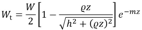
where Wt is the tunnel cross-sectional sound power at distance z, while h is the height of the tunnel, and the surface reflection term ϱ = β0.98. As it results in an estimation of the tunnel cross-sectional sound power, the ASJ model is independent of receiver position in the x, y plane, and the simplification assumes that the source is positioned on the floor of the tunnel. As noted in [26], the ASJ model can incorporate simple variations in surface absorption properties in sections along the tunnel length, by replacing the ϱz terms with ∑ϱizi for the ith section.
The ASJ model as defined in Equation 7 has been implemented in an Excel spreadsheet to calculate the expected sound propagation along the validation test tunnel as before, with the sound power predictions converted to (spatially-averaged) mean-square sound pressure levels LpA using the plane wave (far-field) relationship ![]() , where I is the (time-averaged) sound intensity. The validation results are shown in Figure 13 and Figure 14.
, where I is the (time-averaged) sound intensity. The validation results are shown in Figure 13 and Figure 14.
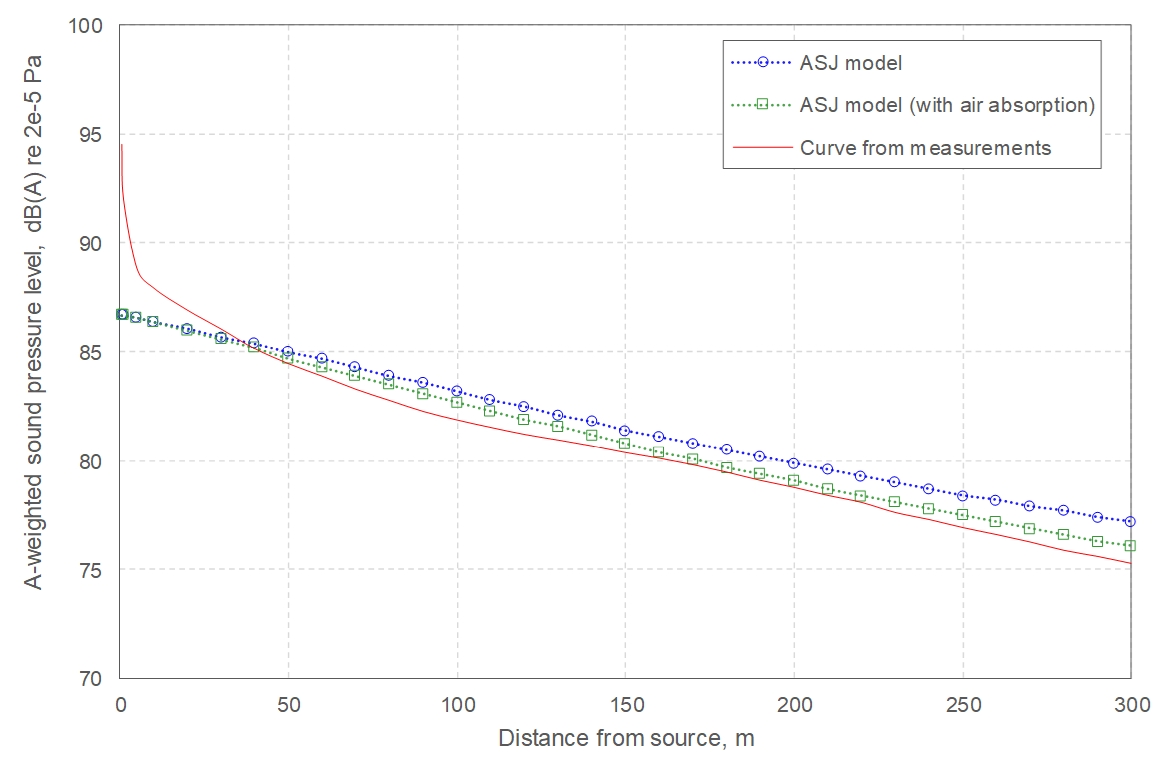
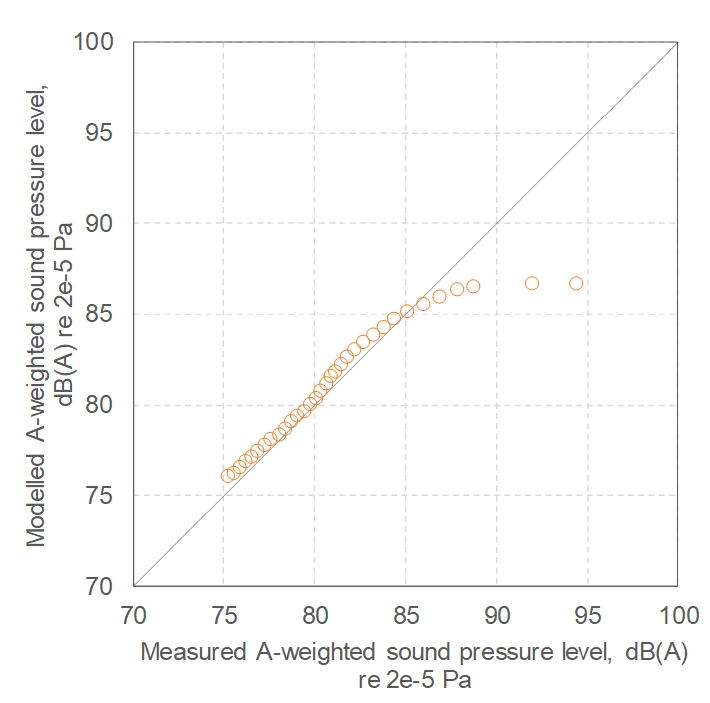
Figure 13 and Figure 14 indicate that, with air absorption included, the ASJ model also predicts values that are reasonably close to the measurements, with errors <2 dB for distances ≥10 m (RMSE = 1.2 dB); within 10m, errors increase to ~8 dB, with systematic under-estimation observed – this is likely a result of the break down in the validity of the plane wave/far-field assumption used to estimate the LpA from the cross-sectional power.
The results above suggest that either the BBN or the ASJ incoherent ISMs are reasonably accurate when applied to omnidirectional sources. However, the ASJ model, which is considerably simpler to implement, includes no facility to characterise the directionality of the source.
Coherent image source method
A coherent image source model for tunnels and long rooms was developed by Iu[32] and Li[33] based on theoretical work by Lemire and Nicolas[34]. The geometrical definitions are very similar to the incoherent models described above, with phase angle changes at each specular reflection included using a complex surface admittance and spherical wave reflection coefficient. The total sound field at a receiver point is calculated as the sum of the complex pressure wave paths from all (real and image) sources. Since the method again computes each individual image source path, it would be possible to incorporate the effects of source directivity, although the model’s original formulation does not accommodate this.
Test comparisons with measurements made in scale model and real tunnels indicated good agreement with predicted narrowband spectra[32][33][35], and with third-octave band levels. The model was later extended to include diffuse reflections using analytical expressions to represent the portions of energy diffusely reflected (ie scattered) at each reflection from roughened surfaces[36].
Comparison of the incoherent and coherent ISM calculations made in [32] suggests that, when considering sound in third-octave bandwidths i) the coherent model tended to predict slightly greater attenuation (ie lower absolute levels), as well as greater variation in level along the tunnel length, and ii) that predictions with incoherent models tended to be within a few dB of the coherent model predictions. While it must be recognised that the coherent model theoretically represents the physical nature of the situation more faithfully, there are also drawbacks: i) increased computational expense, as multiple frequencies must be calculated individually before combining results into wider bandwidths, and ii) the need to acquire or estimate input parameters in narrowband spectral resolution, which are not usually available. Although estimations are possible to interpolate from typical test data and known analytical relationships, this would inevitably introduce uncertainty into the model that may not be distinguishable from other potential sources of uncertainty. In view of the good agreement obtained in the validation comparison with the tunnel measurement data for the incoherent model, any potential additional accuracy and resolution available in coherent models is not believed to outweigh these disadvantages within the context of the present application.
Diffuse reflection method
As well as presenting an incoherent ISM quite similar to the BBN model, Kuttruff derived an (approximate) analytical method to estimate the sound level for a source and receiver aligned along the central axis of a circular long room with diffusely reflecting surfaces[37]. Kuttruff’s model is based on the ‘radiosity integral’, and assumes Lambertian reflection patterns[38]; it can be expressed as follows (for an omnidirectional source, disregarding air absorption):
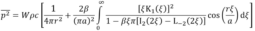
where a is the radius of the cross-section, I2 is the 2nd-order hyperbolic (modified) Bessel function of the first kind, K1 is the 1st-order hyperbolic (modified) Bessel function of the second kind, and L-2 is the modified Struve function (order: -2)[37].
Numerical integration of Equation 8 using the same input parameters as before yields the result shown in Figure 15. Figure 15 is especially notable for two reasons: i) it supports the finding already indicated using the ISM that the tunnels in question are best represented by a specular reflection model, and ii) it indicates that significant attenuation might be achieved by the introduction of numerous scattering surfaces inside the tunnel. This is important because, while installing absorptive materials may be one obvious way to lower sound levels emitted from tunnels, many porous absorptive materials are unsuitable for such environments, which often carry relatively high levels of air particulates and may be difficult to maintain to avoid impaired performance – scattering surfaces on the other hand can be imperforate and therefore would require less maintenance in such an environment. To achieve optimum performance using such an approach, the ‘roughness’ of the scattering surfaces would need to be of sufficient depth to ensure that all wavelengths of significance in the source emission spectrum would be effectively scattered.
3D Geometrical acoustics hybrid method
In this section, a tunnel model is presented based on a 3D geometry, which has been used with the geometrical acoustics modelling software Odeon (v11[39]). One other previous study validated the use of Odeon in predicting sound levels at close range around a train car inside a circular tunnel[40], while another validated its use in predicting room acoustics parameters such as reverberation time and speech transmission index within underground stations[41], but neither tested the sound propagation in tunnels over the longer ranges considered here.
The main advantage of using a 3D model is the ability to explore the influence of the geometry, as well as greater flexibility in surface property assignments (eg for design purposes). Source directivity can also be straightforwardly incorporated and is not limited to rotational symmetry. The potential disadvantage is the greater number of input parameters, which must be carefully considered in relation to validating and calibrating any model.
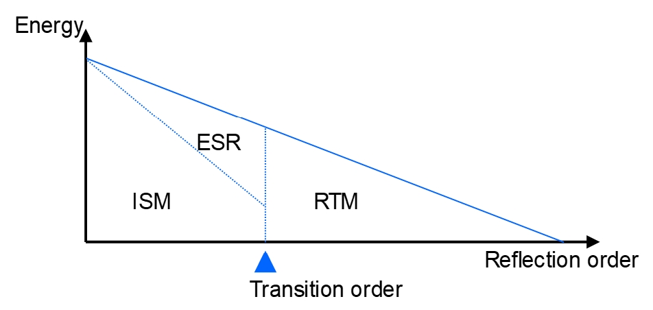
Odeon employs a hybrid approach that combines the ISM with ray-tracing and radiosity methods (see [10] for theoretical background). The manner in which these methods are combined is shown as a schematic diagram in Figure 16. In general, the early part of the reflection model is separated into the (specular reflection) ISM and the ‘early scattering rays’ (ESR), which are modelled using ray-radiosity – these methods are used up to the ‘transition order’ (TO), which is a parameter defining the number of reflection orders before a sound ray transitions to the late reflection model. The late reflections are modelled using the ray-tracing method (RTM), which incorporates scattering[42]. The TO therefore controls the balance between the application of the ISM and the RTM in the model.
Another key set of parameters related to the TO is the number of rays used in the model – the ‘early rays’ are used to identify valid image sources in the ISM part of the reflections, while the ‘late rays’ are used in the RTM part. If a high TO is used (delaying the onset of the RTM part), then the number of early rays would need to be increased and late rays could be reduced (and vice versa). Unless manually altered, the software automatically adjusts the numbers of early and late rays according to recommended values corresponding with the selected TO.
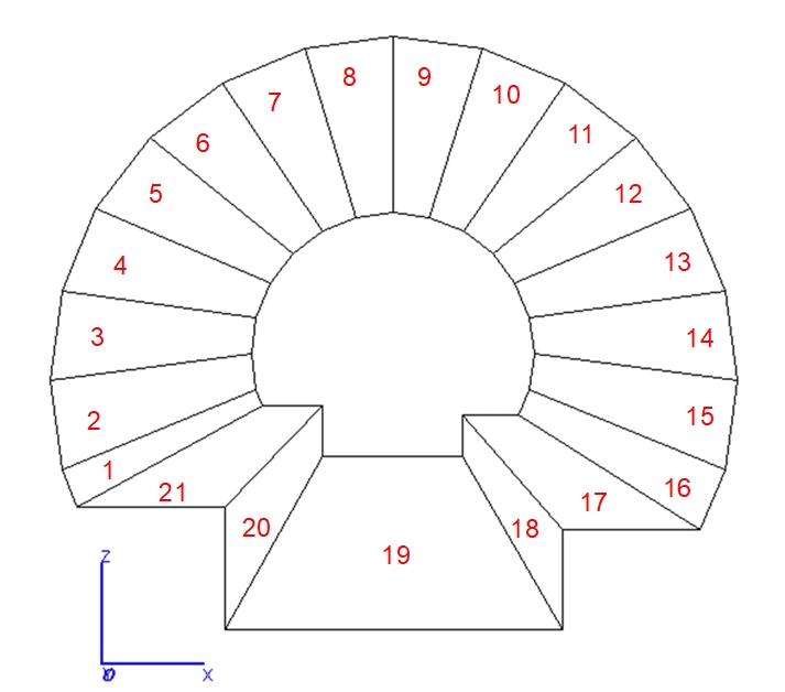
The 3D geometrical model must be constructed using flat polygons, which means that any curved surfaces must be tessellated. Naturally, the tessellation resolution is a variable of interest in modelling a cylindrical tunnel – for the reasons identified in the discussion below, a tessellation of 16 planes was used to divide the curved section of the tunnel surface, as indicated in the diagram in Figure 17 (NB: the Odeon model coordinate system is oriented such that the y-axis is parallel with the tunnel axis). The tunnel length used was 400m, with the source situated at 50m along the tunnel axis.
There are two types of scattering considered in the Odeon model: i) ‘roughness scattering’ caused by the irregularities of the surface material – this is controlled by the scattering coefficient, a parameter which is effectively independent of the surface dimensions, and ii) ‘edge-diffraction scattering’, caused by the finite size of each surface. Both scattering types are frequency-dependent – the roughness scattering coefficient is a single numerical input value that is automatically extrapolated to a pre-defined scattering spectrum, while the edge-diffraction scattering depends on the surface size relative to the wavelength [39]. The tessellation of curved surfaces therefore influences the amount of edge-diffraction scattering occurring, which would represent an artificial increase in scattering caused by the division of a single surface into multiple polygons. This anomaly is addressed in Odeon by designating curved surfaces as a ‘fractional’ type, which ensures the calculation does not include edge-diffraction scattering based on the tessellated polygon sizes [39].
The parametric setup for the model was developed by investigating the effects of varying the values in a systematic manner and ‘calibrating’ the model to more closely represent the measurements. The key settings established in this way are shown in Table 3, and the effects of their variation is discussed below – unless otherwise indicated, the settings used in each calculation took the values in Table 3. It should be noted that Odeon automatically includes air absorption effects, the parameters for which have been set in consistency with the calculations described above.
| Parameter | Value |
|---|---|
|
Transition order |
10 |
|
Number of early rays |
757248 |
|
Number of early scatter rays per image source |
100 |
|
Number of late rays |
25000 |
|
Number of reflections |
2000 |
|
Impulse response length |
25 (s) |
|
Edge-diffraction scattering |
Enabled – surfaces 1-18 and 20-21 as fractional (surface 19: normal) |
|
Surface roughness scattering |
Surfaces 1-18 and 20-21 (Figure 17): 0% Surface 19 (trackbed, Figure 17): 5% |
|
Surface absorption coefficients |
Tunnel surfaces: Table 2 Tunnel ends: 100% absorptive |
|
Curved surface tessellation |
16 planes |
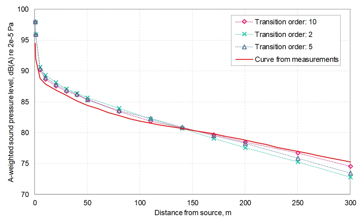
The effect of varying the TO is shown in Figure 18. For the calculation in Figure 18, the number of early and late rays were manually held constant to explicitly show the effect of TO variation in isolation. The manually-selected numbers of a) early and b) late rays were respectively based on a) the Odeon-recommended value for a TO of 10 (the maximum TO value allowed), and b) a value much larger than the Odeon-recommended value.
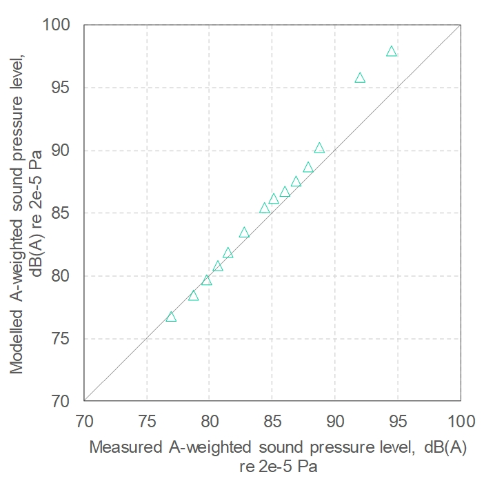
Figure 18 and Figure 19 indicate that: i) the 3D Odeon model is capable of predicting the measured values with good accuracy similar to that observed using the BBN ISM model, and ii) the best agreement with measurements was achieved by increasing TO, ie by maximising the ISM part of the model. This had the effect of increasing the sound levels propagated to longer range, and slightly reducing the levels at shorter range, with an apparent inflexion point at around 150m from the source.
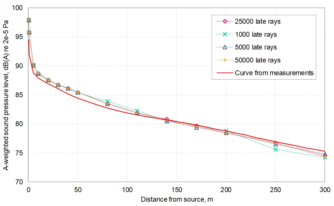
The effect of varying the number of late rays (using constant TO and early ray number) is shown in Figure 20. Figure 20 shows that the late ray number has a smaller effect (which is expected, given the minimisation of the RTM part of the model), and the results appear to converge around 25000 rays.
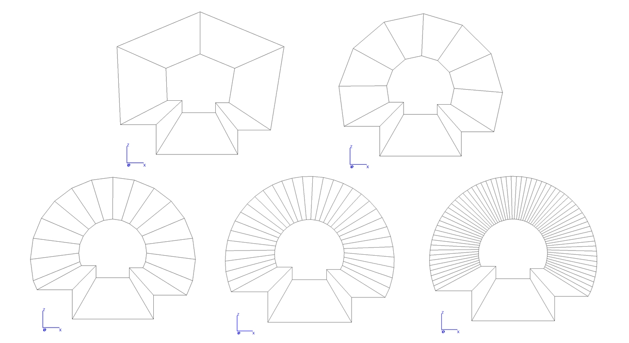
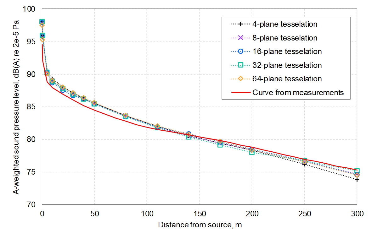
The tessellation of the curved tunnel surface was varied in 5 resolutions from 4 to 64 planes, as shown in Figure 21; it should be noted that, due to the variation in geometry, the cross-sectional areas of the models varied slightly from about 36.4-37.5 m2, which may also have a small effect on the corresponding calculations.
The effects of varying the resolution in this way is shown in Figure 22. In this calculation, the number of early rays was increased to 1,290,752 for all the resolutions, which was the Odeon-recommended value for the 64-plane tessellation.
Interestingly, Figure 22 indicates that the resolution of the curved surface tessellation had only a very minor effect on the predicted sound levels, which is consistent with the earlier finding that the rectangular tunnel ISM BBN model predicted the levels with reasonable accuracy. From this it may be surmised that, for specular reflections with low absorption (and negligible scattering) the cross-sectional shape of the tunnel is of little importance in comparison with its overall dimensions – at least, as far as the incoherent energy propagation model is concerned; it is possible that coherent models examining localised sound field variations within the tunnel may highlight differences that become visible in narrowband spectra.
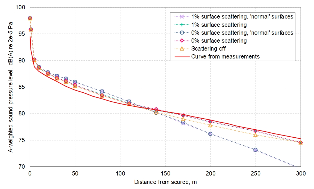
The scattering setup was explored in two ways: i) the designation of surfaces as ‘fractional’ or ‘normal’ was varied to examine the effect on edge-diffraction scattering, and the surface scattering coefficient was also varied slightly to investigate the possible influence of roughness scattering; the results are shown in Figure 23. It should be noted that in Figure 23, the results indicated as ‘normal’ represent a setup in which only the curved surfaces (ie surfaces 1-16 as shown in Figure 17) are designated as ‘fractional’ – this is the normal way an Odeon model would be set up for this situation. The results in Figure 23 not designated as ‘normal’ applied the fractional surface designation to the curved surfaces and to the four walkway surfaces (17-18 and 20-21 as shown in Figure 17), but not to the trackbed surface (19 as shown in Figure 17) – in this way edge-diffraction was further reduced in the model beyond what would normally be the case.
Figure 23 illustrates some interesting findings: both sets of results using the ‘normal’ edge-diffraction setup yielded relatively large errors, diverging from the measurements with increasing distance. When the walkway surfaces were also designated as fractional (despite not being part of the curved surface), this effect was significantly reduced, and the results more closely agreed with measurements. This indicates that scattering due to edge-diffraction must be minimised in this type of model, to ensure that the attenuation with distance is not over-estimated. The small variation in the surface scattering coefficient had a negligible effect on the results, while turning all scattering ‘off’ (ie disabling edge-diffraction scattering and surface roughness scattering) resulted in increased error compared with measurements; this indicates that the tunnel model is most accurate with some scattering included, but it should be limited to the trackbed – the geometrical polygonal model omits the trackform, which in reality would be expected to scatter rays encountering this surface.
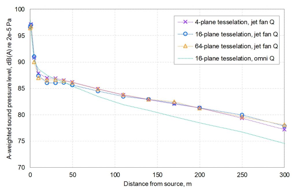
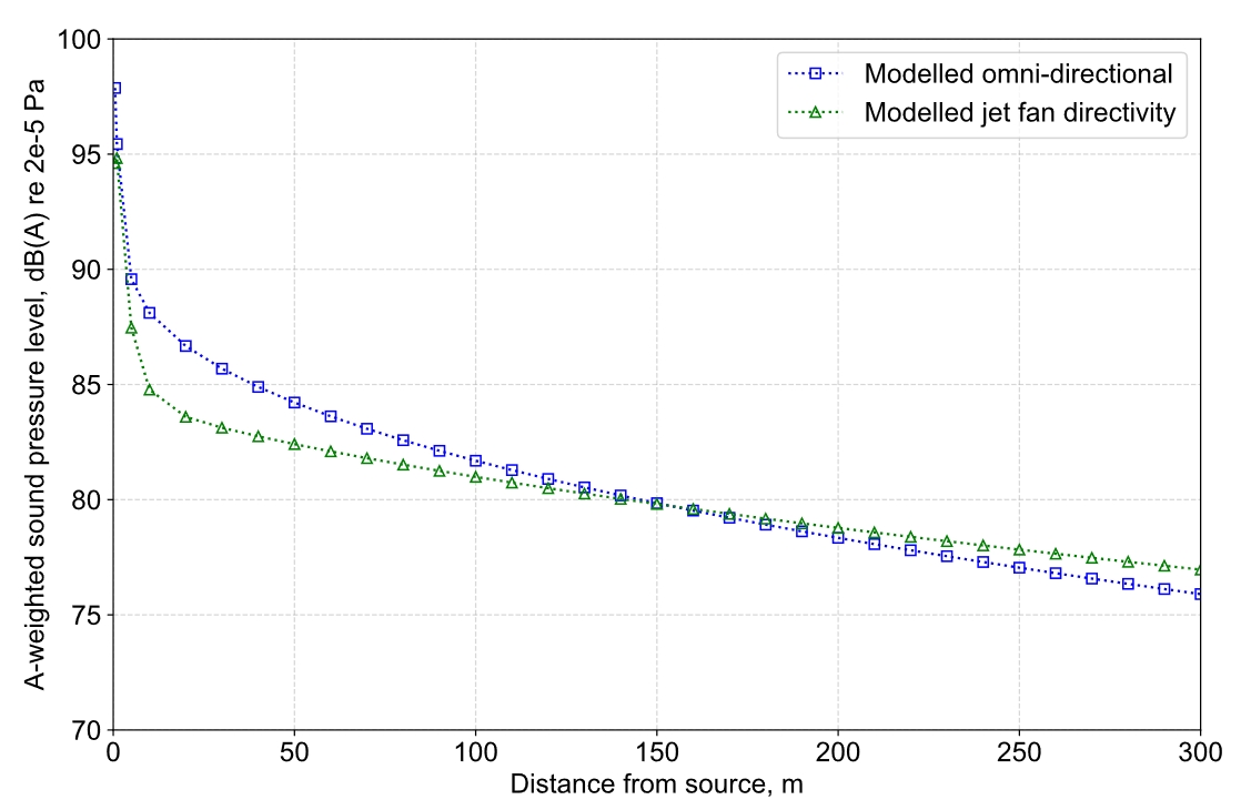
The jet fan source directivity characteristic in Figure 2 has been applied in the 3D model to further investigate the jet fan sound propagation, as shown in Figure 24. Figure 24 supports the earlier observation made using the BBN model that the jet fan source directivity may result in increased sound levels at longer ranges along the tunnel. However, comparison of Figure 24 with Figure 12 shows that the observed effect is stronger in the 3D model, resulting in a difference of up to 3 dB compared with the omnidirectional source. The 3D model more closely represents the actual tunnel geometry, so is considered likely to be a more accurate prediction of the actual jet fan behaviour that might be encountered. The observed ‘dip’ in level at closer range (attributable to the influence of the off-axis direct field contribution) is also again observed, although it is much less pronounced than predicted using the BBN model. The results in Figure 24 are given for three of the curved surface tessellations, to examine whether the resolution of the geometry has more of an effect on the propagation from a directional source than an omni-directional one (all other settings were as per Table 3) – Figure 24 shows relatively small differences between the resolutions, ie <2 dB, which is similar to the estimations for the omni-directional source.
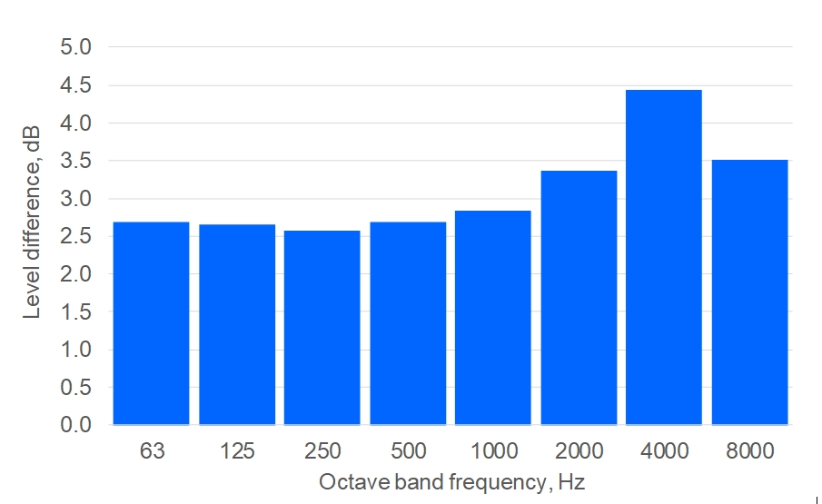
The results in Figure 24 indicate that application of the ASJ model (which does not incorporate source directivity) to jet fan sound emissions from tunnels may result in underestimations of the levels propagated to the tunnel openings. At ranges of up to 300m, the difference in the overall A-weighted levels could be expected to reach up to ~3 dB. This suggests that the simpler ASJ model could be used to make conservative estimations of jet fan sound propagation provided that a margin for source directivity is added to the predicted level. The analysis so far has focussed on the overall A-weighted levels, however, to avoid dependence on the particulars of the source spectrum, level differences between the models should be expressed in separated frequency bands. The calculated octave band level differences between the 3D model predictions (including jet fan source directivity), and the ASJ model predictions (omni-directional source, approximately converted to sound pressure using the far-field relationship as before), are shown in Figure 25. Figure 25 indicates that, at ranges ≥10m the octave band level differences are within a range of around -1 to 4 dB.
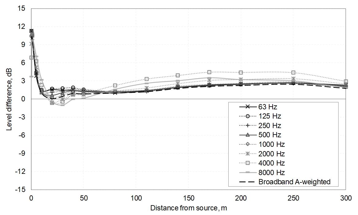
The maximum positive level differences over this distance range are shown in Figure 26. The addition of the numerical values in Figure 26 to calculations made using the ASJ model would ensure the predicted levels are no lower than those calculated using the 3D geometrical model.
Conclusions and recommendations for further work
The BBN ISM model for tunnel sound propagation has been validated against available measurement data for a cylindrical railway tunnel and an omni-directional source. The simplified ASJ model (based on the ISM) has also been validated against the same measurement data.
Empirical data from measurements of jet fan sound have been used to derive an estimate of frequency-dependent source directivity patterns. These directivity patterns have been used in conjunction with the validated BBN model to predict jet fan source-specific propagation in the tunnel, the results of which indicate that increased levels at longer ranges may be expected, compared with an omni-directional source.
The 3D geometrical acoustics (hybrid ISM-radiosity-ray-tracing) modelling tool Odeon has been used to verify the observation that jet fan source directivity may increase levels of tunnel sound propagation, the results of which showed that the introduction of jet fan directivity resulted in a ~3 dB increase in A-weighted levels compared with an omni-directional source at ranges of up to 300m (a more pronounced effect than observed using the more simplistic BBN model). Spectral separation into octave bands indicates this difference varies in the range 2.6 to 4.4 dB (mean value: 3.1 dB). This suggests that a corresponding margin could be added to the ASJ model results to give reasonably conservative estimations of jet fan tunnel sound propagation, although it is acknowledged that jet fan directivity patterns in general will vary from the behaviour assumed here, which would affect the validity of this suggested margin.
The validation of the 3D geometrical acoustics model against measurements is believed to represent the first published result to demonstrate the applicability and validity of the Odeon tool to railway tunnel sound propagation over long ranges. The good agreement with the measurements is predicated on the maximisation of the ISM part of the model and the corresponding minimisation of the RTM part, and minimisation of the influence of scattering (via edge-diffraction and surface roughness mechanisms). In other words, the use of a tool such as Odeon with a ‘standard’ setup could result in inaccurate estimations of tunnel sound propagation, which appears to be mainly linked to overestimation of the attenuation caused by scattering. Accordingly, careful calibration of the model setup was found to be necessary to obtain good agreement with measurements. In the absence of measurements available to calibrate such a model, the ISM of the BBN model appears to exhibit remarkably high accuracy, in view of its simplifications and geometrical approximations. However, this approach lacks some of the other benefits of a 3D geometrical tool, such as flexibility in the design and placement of surface treatments, and geometric variations.
Results of calculations made using a model incorporating diffuse reflections suggest that high scattering (which may be caused by surface roughness or by edge-diffraction associated with small surface areas) will lead to significant attenuation along the length of a tunnel. This indicates that design consideration of surface treatments used to reduce noise emitted from a tunnel should not be limited to absorptive materials, which often raise difficult problems relating to maintainability; imperforate surface treatments designed to maximise scattering could yield significant noise reductions, provided the important sound wavelengths are taken into account in determining the scattering dimensions.
Although not discussed here, approaches to estimating the directivity of sound emissions from the tunnel mouth opening (which exhibits non-uniform directivity and thus will influence the level of jet fan sound impacting noise-sensitive receptors) have also been researched, with examples of numerical analyses[43], extrapolations of empirically-based standardised prediction methods[44], scale model experiments[28] [29][45] and field studies [30] reviewed. Further work is necessary to distil the available research into a rationalised representation relevant to the application.
Acknowledgements
The assistance of Erich Thalheimer (WSP) and Mark Gilbey (WSP) is gratefully acknowledged.
References
| Title | |
|---|---|
|
[1] |
P. Ridley and D. Spearritt, “Evaluation of speech transmission in a road tunnel,” in Proceedings of Acoustics 2011, 2-4 November, Gold Coast, Australia, 2011. |
|
[2] |
C. Richardson and B. Weyers, “The Clem7 motorway tunnel: mechanical and electrical plant acoustic design and performance,” in Proceedings of Acoustics 2011, 2-4 November, Gold Coast, Australia, 2011. |
|
[3] |
J. Kang, “Reverberation in rectangular long enclosures with geometrically reflecting boundaries,” Acta Acustica united with Acustica, vol. 82, no. 3, pp. 509-516, 1996. |
|
[4] |
E. Thalheimer, R. Greene and J. Poling, “Fan manufacturer sound power data – trust but verify,” in Noise-Con 2016, 13-15 June, Providence, USA, 2016. |
|
[5] |
D. A. Bies, C. H. Hansen and C. Q. Howard, Engineering noise control, 5th ed., Boca Raton: CRC Press, 2018. |
|
[6] |
J. L. Davy, “The directivity of the sound radiation from panels and openings,” Journal of the Acoustical Society of America, vol. 125, no. 6, pp. 3795-3805, 2009. |
|
[7] |
M. Hodgson, “When is diffuse-field theory applicable?,” Applied Acoustics, vol. 49, no. 3, pp. 197-207, 1996. |
|
[8] |
W. C. Sabine, Collected paper on acoustics, Cambridge: Harvard University Press, 1922. |
|
[9] |
J. Kang, Acoustics of long spaces, London: Thomas Telford, 2002. |
|
[10] |
L. Savioja and U. P. Svensson, “Overview of geometrical room acoustic modeling techniques,” Journal of the Acoustical Society of America, vol. 138, no. 2, pp. 708-730, 2015. |
|
[11] |
A. D. Pierce, Acoustics: an introduction to its physical principles and applications, 3rd ed., Cham: Springer Nature, 2019. |
|
[12] |
J. B. Allen and D. A. Berkley, “Image method for efficiently simulating small-room acoustics,” Journal of the Acoustical Society of America, vol. 65, no. 4, pp. 943-950, 1979. |
|
[13] |
E. A. Lehmann and A. M. Johansson, “Prediction of energy decay in room impulse responses simulated with an image-source model,” Journal of the Acoustical Society of America, vol. 124, no. 1, pp. 269-277, 2008. |
|
[14] |
F. Mechel, Room acoustical fields, Berlin: Springer-Verlag, 2013. |
|
[15] |
J. Sheaffer, “From source to brain: modelling sound propagation and localisation in rooms,” University of Salford (PhD thesis), Manchester, 2013. |
|
[16] |
M. Vorländer, “Computer simulations in room acoustics: concepts and uncertainties,” Journal of the Acoustical Society of America, vol. 133, no. 3, pp. 1203-1213, 2013. |
|
[17] |
P. Economou and P. Charalampous, “Room resonance using wave based geometrical acoustics (WBGA),” in ICSV23, 10-14 July, Athens, Greece, 2016. |
|
[18] |
P. M. Morse and K. U. Ingard, Theoretical acoustics, New York: McGraw-Hill, 1968. |
|
[19] |
U. Bolleter and R. C. Chanaud, “Propagation of fan noise in cylindrical ducts,” Journal of the Acoustical Society of America, vol. 49, no. 3, pp. 627-638, 1971. |
|
[20] |
I. R. Kinghorn and A. F. Green, “Jetfan selection and design report 588-RUG-RDRAK-00179-00,” Channel Tunnel Rail Link, 2007. |
|
[21] |
H. W. Bobran, Handbuch der bauphysik (Handbook of building physics), Berlin: Verlag Ulstein, 1973. |
|
[22] |
ISO, “ISO 9613-1:1993 Acoustics – Attenuation of sound during propagaion outdoors – Part 1: Calculation of the absorption of sound by the atmosphere,” International Standards Organisation, Geneva, 1993. |
|
[23] |
B. M. Gibbs and D. K. Jones, “A simple image method for calculating the distribution of sound pressure levels within an enclosure,” Acustica, vol. 26, no. 1, pp. 24-32, 1972. |
|
[24] |
A. G. Galaitsis and W. N. Patterson, “Prediction of noise distribution in various enclosures from free-field measurements,” Journal of the Acoustical Society of America, vol. 60, no. 4, pp. 848-856, 1976. |
|
[25] |
Y. Kobayashi, S. Seki, T. Kitamura, K.-I. Mitsui and S. Yamada, “Study on the characteristics of noise propagation in tunnel and noise control with absorbing material of ceramics,” in Proceedings of Inter-noise 1999, 6-8 December, Fort Lauderdale, USA, 1999. |
|
[26] |
T. Miyake, K. Takagi, K. Yamamoto, H. Tachibana and H. Iimori, “トンネル坑 口周辺部の騒音予測法について (Study on prediction of road traffic noise around tunnel entrance),” Journal of the Institute of Noise Control Engineering of Japan, vol. 24, no. 2, pp. 127-135, 2000. |
|
[27] |
K. Takagi, T. Miyake, K. Yamamoto and H. Tachibana, “Prediction of road traffic noise around tunnel mouth,” in Proceedings of Inter-noise 2000, 27-30 August, Nice, France, 2000. |
|
[28] |
H. Tachibana, S. Sakamoto and A. Nakai, “Scale model experiment on sound radiation from tunnel mouth,” in Proceedings of Inter-noise 1999, 6-8 December, Fort Lauderdale, USA, 1999. |
|
[29] |
S. Sakamoto, “トンネル坑口からの音響放射に関する縮尺模型実験 (Scale-model experiment on sound radiation characteristics from a tunnel portal),” The Journal of the Acoustical Society of Japan (J), vol. 74, no. 2, pp. 63-71, 2018. |
|
[30] |
S. Sakamoto, T. Matsumoto and O. Funahashi, “Validation of calculation method of tunnel portal noise in ASJ RTN-Model 2018 by a field experiment,” Acoustical Science and Technology, vol. 41, no. 3, pp. 614-621, 2020. |
|
[31] |
S. Sakamoto, “Road traffic noise prediction model “ASJ RTN-Model 2018”: Report of the Research Committee on Road Traffic Noise,” Acoustical Science and Technology, vol. 41, no. 3, pp. 529-589, 2020. |
|
[32] |
K. K. Iu, “The prediction of noise propagation in street canyons and tunnels,” The Hong Kong Polytechnic University (MPhil thesis), 2003. |
|
[33] |
K. M. Li and K. K. Iu, “Propagation of sound in long enclosures,” Journal of the Acoustical Society of America, vol. 116, no. 5, pp. 2759-2770, 2004. |
|
[34] |
G. Lemire and J. Nicolas, “Aerial propagation of spherical sound waves in bounded spaces,” Journal of the Acoustical Society of America, vol. 86, no. 5, pp. 1845-1853, 1989. |
|
[35] |
K. M. Li and K. K. Iu, “Full-scale measurements for noise transmission in tunnels,” Journal of the Acoustical Society of America, vol. 117, no. 3, pp. 1138-1145, 2005. |
|
[36] |
M. K. Law, K. M. Li and C. W. Leung, “Noise reduction in tunnels by hard rough surfaces,” Journal of the Acoustical Society of America, vol. 124, no. 2, pp. 961-972, 2008. |
|
[37] |
H. Kuttruff, “Stationare Schallausbreitung in Langraumen (Stationary sound propagation in long rooms),” Acustica, vol. 69, no. 2, pp. 53-62, 1989. |
|
[38] |
H. Kuttruff and E. Mommertz, “Room Acoustics,” in Handbook of Engineering Acoustics, G. Müller and M. Möser, Eds., Berlin, Springer-Verlag, 2013, pp. 238-267. |
|
[39] |
C. L. Christensen, “ODEON room acoustics software. Version 11. User Manual, 2nd edition.,” Odeon A/S, Lyngby, 2011. |
|
[40] |
T. Kors, K.-R. Kirchner, D. Fast, A. Vallespin, J. Sapena, A. G. Garcia and O. Martner, “Sound propagation and distribution around typical train carbody structures,” in Euronoise 2018, 27-31 May, Crete, Greece, 2018. |
|
[41] |
L. Gomez-Agustina, “Design and optimisation of voice alarm systems for underground stations,” London South Bank University (PhD thesis), London, 2012. |
|
[42] |
C. L. Christensen and J. H. Rindel, “A new scattering method that combines roughness and diffraction effects,” in Forum Acusticum, 29 August – 2 September, Budapest, Hungary, 2005. |
|
[43] |
J. Hübelt, C. Schulze, K. S and W. Bartolomaeus, “A German Prediction Model of the Sound Propagation in and around tunnels,” in Inter-noise 2012, 19-22 August, New York, USA, 2012. |
|
[44] |
W. Probst, “Prediction of sound radiated from tunnel openings,” Noise Control Engineering Journal, vol. 58, no. 2, pp. 201-211, 2010. |
|
[45] |
K. Heutschi and R. Bayer, “Sound radiation from railway tunnel openings,” Acta Acustica united with Acustica, vol. 92, no. 4, pp. 567-573, 2006. |
Peer review
- Mark HowardChief Engineer, HS2 Ltd