The use of remote sensing to identify habitats on a large-scale linear infrastructure project

Introduction

MWJV, a joint venture comprising Mott Macdonald and WSP, was appointed to undertake an Environmental Impact Assessment (EIA) of the Western Leg (Crewe to Manchester), Phase 2b of the High Speed Two (HS2) Proposed Scheme. The EIA and formal Environmental Statement (ES) will accompany the deposit of the Phase 2b hybrid Bill in Parliament. As part of the EIA work, ecology and biodiversity forms one of many environmental topic areas that is considered in the technical scope for where likely significant effects of the Proposed Scheme are assessed.

The starting point of all ecological assessment often begins with the identification of habitats within areas affected by the Proposed Scheme and within the Zone of Influence^[1]. This is usually undertaken as part of Preliminary Ecological Appraisals (PEA)^[2] whereby Phase 1 Habitat Survey^[3] forms part of the methodology. HS2 follow recognised industry best practice methodologies for the purposes of baseline data collection to inform assessment and these are outlined in a Scope and Methodology Report (SMR)^[4] and Field Surveys Methods and Standards (FSMS) Technical Note^[5]. The SMR and FSMS require habitat mapping to be undertaken within land required for the construction of the Proposed Scheme and up to 500m from this boundary. Whilst habitat mapping is required within the 500m buffer, the FSMS specifies variations of methodology to be used in each zone extending from the central zone. These are summarised as follows and is shown in Figure 1:

• Land required for the construction of the Proposed Scheme and 100m either side: Full extended Phase 1 Habitat Survey;
• Within the zone extending to a further 150m (i.e. 101-250m from the boundary of the land required for the construction of the Proposed Scheme): Standard Phase 1 habitat survey; and
• From 250m to 500m from the boundary of land required for the construction of the Proposed Scheme: Habitats mapped from aerial photograph interpretation alone with no requirement to undertake a field-based Phase 1 habitat survey.

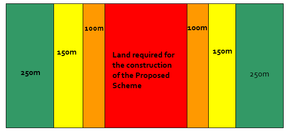
The requirement for Phase 1 habitat mapping for the entire route of the Proposed Scheme and within the survey buffers shown in Figure 1 is a clear deliverable of the Ecology and Biodiversity technical scope. The scale of this exercise, when put in context of the size, complexity and magnitude of HS2, presents significant challenges to overcome when delivering a consistent and accurate digitised habitat map over a large linear area.

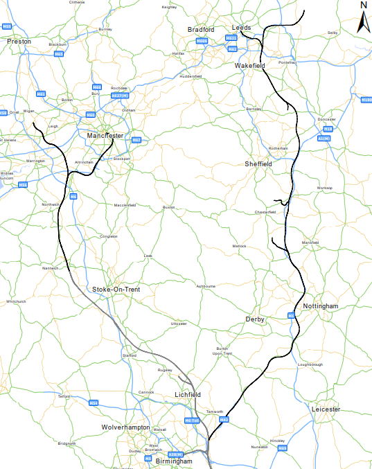
The Western Leg of Phase 2b connects Crewe to Manchester and extends approximately 85km in length. The extent of land required for the construction of the Proposed Scheme is variable along the route and is often dependent on the type of infrastructure design, ancillary works, utilities and construction methodologies. For example, the width of land required for the construction of the Proposed Scheme can extend over 1km where large box structures or maintenance sidings are being considered, whilst it can contract to 45m where viaduct crossings are being designed. Habitat mapping was required across approximately 117km² of land for the Western Leg.

A classification method to pick out varying habitat typologies (vegetation and other physical features) using remote sensing data and other digital datasets was developed in order to overcome issues associated with mapping such an extent. Following initial modelling work and production of habitat map outputs using this method for the Western Leg, HS2 instructed MWJV to undertake the habitat classification method for the Eastern Leg, which extends from the West Midlands to Leeds with a total route length of 198km. The area requiring the mapping of habitats within the Eastern Leg was approximately 344km², which took into account the land required for construction of the Proposed Scheme and associated buffers shown in Figure 1.

This paper discusses the need for an automated digital approach and the evolution of a methodology used to classify habitats prior to field survey work. The combined area that required habitat mapping for Phase 2b, including the Western and Eastern Legs, totalled approximately 461km².

Phase 1 Habitat Survey

Phase 1 habitat survey is a widely recognised habitat classification system^[6] published by the UK Joint Nature Conservation Committee (JNCC)^[3]. The JNCC methodology assigns habitat types from a specified list, and maps are produced using standard colour and letter codes. This methodology seeks to provide relatively rapidly, a record of the semi-natural vegetation over large areas of countryside^[3]. As such, in the development sector, it is widely used and accepted as an approach to define the habitat baseline for nature conservation purposes and to identify further requirements for detailed habitat or species-specific survey^[2]. It also informs decision making in relation to design, impact assessment, mitigation, compliance and licensing.

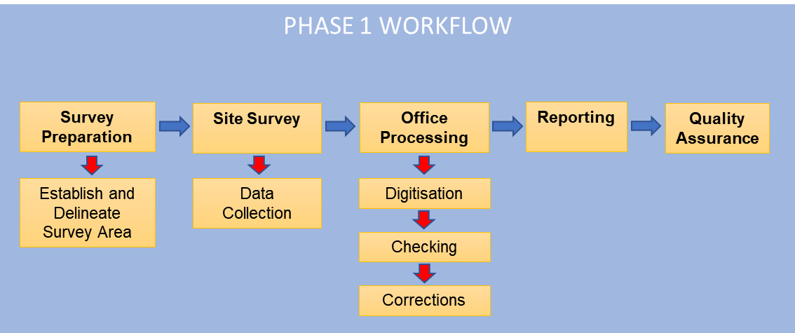
Typically, the workflow to complete a standard Phase 1 habitat survey will start with a trained ecologist visiting all parcels of land within a given survey area and mapping vegetation types on to Ordnance Survey maps, usually at a scale of 1:10,000^[3]. Traditionally, this would be done on paper in the field, manually scribing and assigning JNCC typology to recorded habitats with associated target notes. This would then be processed in the office, digitised and compiled on computers. The end products of a Phase 1 survey being a habitat map, target notes, species lists and a descriptive and interpretive report. Variations on this traditional workflow has more recently seen a move to digital data capture. Digital data capture methods using tablets and various software products facilitates data entry directly into the digital environment and the use of Geographical Information Systems (GIS) permits spatial data and geographically referenced data to be collected^[7]. However, in terms of mapping the types and extents of habitats on GIS systems in the field, these would typically be derived through creating freehand shapefiles against a relevant base map on a tablet. Whilst this is likely to greatly reduce time required for data entry and further processing, significant work would be required to get a clean and presentable dataset as an output for the habitat map^[8]. The typical Phase 1 habitat survey workflow is illustrated in Figure 3.

The origins of Phase 1 habitat survey dates back to the 1970s, when the Nature Conservancy Council (NCC) had a requirement to map wildlife habitats over large areas of countryside^[3]. As this method is still widely used in a planning and assessment context because of it being simple and intuitive, it is applied to specific sites by ecologists as a tool to assess impacts of a proposed scheme. This application does not align with the intentions of the original methodology and as a consequence, inaccuracies, inefficiencies and misclassifications often result. Challenges associated with applying Phase 1 methodology in the context of large-scale linear infrastructure projects are summarised in Table 1.

Challenge	Context
Access and Health and Safety	Patchy access availability due to permissions or health and safety reasons across large linear projects results in data gaps and incomplete coverage throughout the route. Time consuming and inefficient mobilisation of surveys based on variable access permissions and land holdings across large survey areas.
Mapping using Aerial Photography	Low confidence levels in habitats mapped using this method to accurately represent the baseline condition, in the absence of survey validation.
Surveyor Consistency	Surveyor inconsistencies and discrepancies may result from: Differing interpretation of methodology and/or habitat types[9]; Subjectivity applied to observations whilst in the field on the extent, type and condition of habitats; Variability in the extent of survey preparation undertaken; and Disproportionate time allocated to survey land parcels based on size rather than habitat complexity.
Accuracy and Homogeneity	Habitats frequently exist in intimate/complex mosaics and with gradual rather than abrupt transitions between habitat types[8]. Minimum habitat units to be mapped at Phase 1 level is usually 0.1ha[3]. This can be significant in the context of important habitats and therefore, uncertainty and inaccuracies in habitat mapping may arise from: Delineating and spatially representing habitats as polygons, points or lines in the field; Differentiating areas of homogenous habitat across large survey extents.
Habitat Accounting and Duplication	In addition to the complexity of habitat boundaries, the manual drawing of shapefiles presents difficulties with accounting for the total area of a site when the end goal is to create a continuous set of shapefiles: Slivers and gaps in the dataset form as a result of drawing shapes in the field or without using snapping or editing shared boundaries without a topology; and Overlapping polygons can occur when manually drawing shapefiles without clipping.
Processing and Data Handling	The typical Phase 1 workflow (Figure 2) requires that the data is reprocessed on return to the office, where the surveyor error-checks the data before entering it into the GIS database. If the survey information is already entered into GIS databases in the field, this data would need to be processed and reviewed ensuring a clean data set is produced and that typographical errors are corrected. Often, the digitisation would be not be done by the ecologist, but by a GIS specialist, which would require further inefficient data handling and thereby increasing margins for error.
Quality Assurance	Formal Quality Assurance (QA) procedures as part of the typical Phase 1 workflow happens with the report deliverable. The report and associated map outputs are reviewed and approved. This end-point review can be less-effective when it is easy for errors to creep into habitat datasets during data processing[8] and subsequently reported on.

Remote Sensing and Habitat Mapping

Incessant investigation and monitoring of all habitats across the UK would be considered necessary in order to obtain information on extents, distribution, condition, species compositions, conservation values and management regimes. This information is however required to support development planning decision-making as well as appropriate site management considerations.

Since the advent of remote sensing techniques, the satellite image interpretation has become a first choice of ecologists for habitats mapping and classification^{[10],[11],[12],[13],[14],[15],[16]}. However, with the advancement of technology and the availability of various satellite datasets in different spatiotemporal ranges, combined with improving interpretation techniques, there has been a significant increase in its application over the last decade. These techniques are used in a range of scenarios resulting in environmental benefit. For example, remote sensing has been used to identify areas of resource exploitation within specific habitats, as well as in the context of generating information on habitat condition to calculate mitigation compensation areas for Net Gain assessments, often a requirement of large infrastructure schemes. A literature search reveals a variety of remote sensing strategies applied to habitat mapping projects spanning a wide range of spatial scales^{[3][17][18][19][20][21][21]}.

Remotely sensed data in the form of aerial photography is commonly used by field ecologists to map habitats. Maps derived from aerial photos were manually interpreted, and further field visits were made to check, validate and if necessary, modify the species composition and maps. Finally, the resultant maps were digitised in GIS. However, this method is not time or cost-efficient. Moreover, manual interpretation of aerial photographs has often been used in studies that do not rely on species data and for sites that are relatively small in extent. The recent advances in remote sensing has revolutionised the entire process for habitat mapping and modelling. Ecologists, as well as scholars, faced with large sites and industry-level assessments, have turned towards the digital processing of medium-to high spatial-resolution satellite imagery such as Landsat Multispectral Scanner (MSS), Thematic Mapper (TM), or Enhanced Thematic Mapper Plus (ETM), Sentinel, Quick bird, World View satellites for more efficient acquisition of environmental information.

Although digital processing of satellite data for habitat mapping is widely used, the traditional image classification suffers shortcomings owing to the non-normality of spectral signatures and overlapping and heterogeneity of the habitats in question. This impact can be greater in the urban green environment, for example, analysis of habitats is frequently hindered by the complex canopy structures and the presence of compound mosaics or transitions of vegetation types. That is the reason why sometimes digital remote sensing products can be criticised for presenting an overly simplistic representation of vegetation, mainly contributed to by historical limitations of satellite data and the ubiquitous use of classification as an information extraction technique.

However, there is a recent change in both of above factors, with the availability and rapid increase in number of commercial and non-commercial satellites facilitating acquisitions of data in increased and various ranges of spatial, spectral and temporal dimensions. Now we have these newfound choices which has raised our ability to conduct ecological monitoring and management, at the same time it has also presented us with the unique challenge of selecting the appropriate data and using a suitable classification technique. This emphasises that the discussions over habitat information abstraction processes over large-area ecosystem management applications, particularly led at industry standards, must therefore start with the review of the remote sensing scene model, and if it can relate to vegetation as a layered, multiscale phenomenon.

At the leading edge would be the studies which have attempted to incorporate detailed vegetation attributes such as taxonomy, age, structure derived from or along with widely available satellite imagery. There is a need for a framework that combines hierarchy theory with elements of the remote scene model. This would present a mechanism for linking information needs with an image processing technique, as well as providing a foundation for communication between ecologists and specialists in remote sensing. Future research should explore the integrated role of new remote sensing instruments and emerging technologies, develop techniques for constructing multiscale vegetation databases over large areas, and test the utility of these databases for supporting habitat area and condition assessment.

This paper describes a robust solution at ecological consultancy standard that was deployed on HS2 Phase 2b. The solution involves combining the potential of satellite imageries, ancillary data, DSM/DTM (Digital Surface Model/Digital Terrain Model) data along with the existing ecological knowledge base to produce very fine scale pre-classified product which can be transferrable across projects.

Datasets

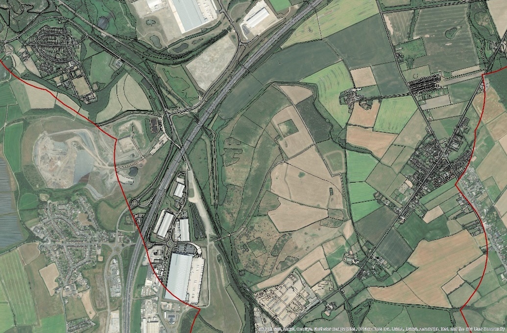
The dataset used in this analysis, encompassing the land required for construction of the Proposed Scheme and associated buffer zones, were provided by HS2 and were captured in 2016.

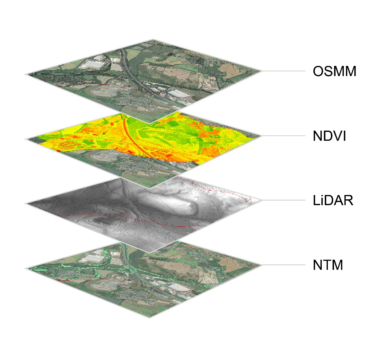
A number of datasets were used for the remote sensing analysis of the HS2 Phase 2b route all with the desired intention to accurately classify habitats. These included:

• Ordinance Survey MasterMap (OSMM)
• Normalised Difference Vegetation Index (NDVI)
• Laser imaging, Detection, and Ranging (LiDAR)
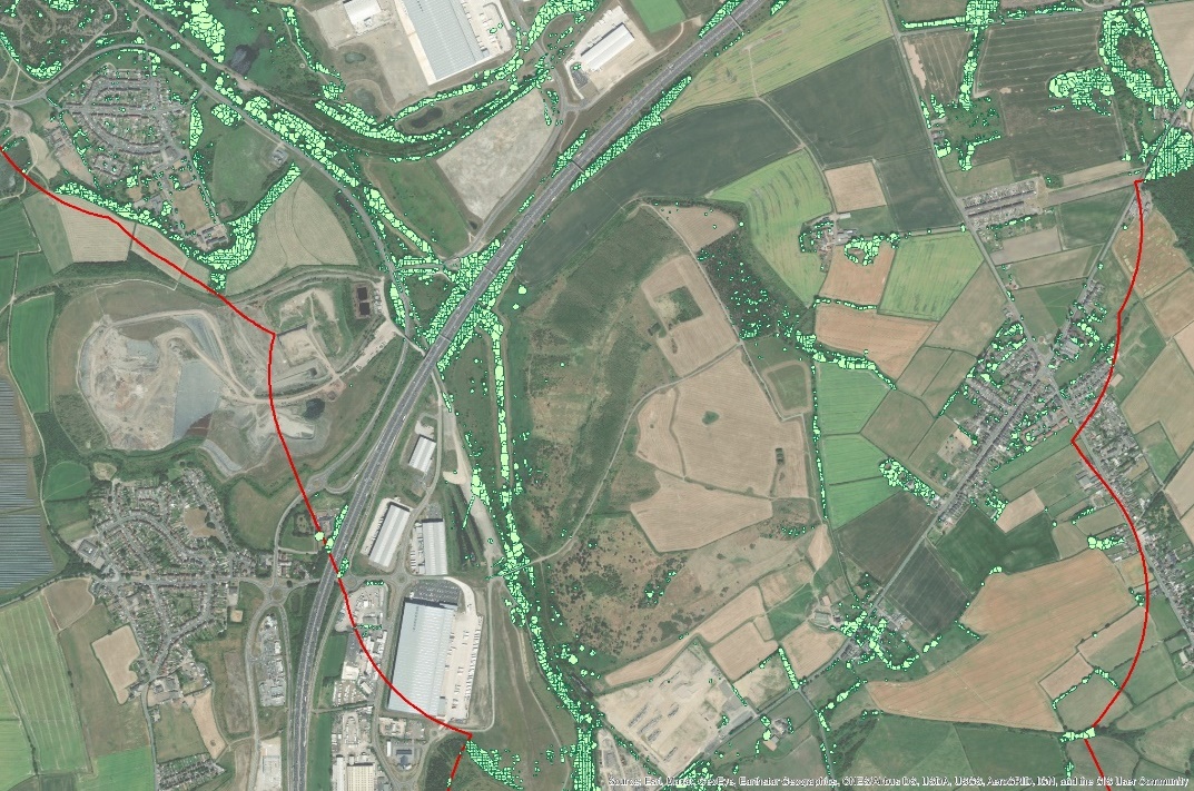
• National Tree Map™ (NTM)

The key dataset in this process was the OSMM vector data (Figure 4). This allowed for the accurate and logical segmentation of the study area into manageable and accurate parcels of land and often habitat delineations to analyse. This also allowed for embedding remote sensing spectral and physical information within the attribute table to facilitate the in-depth multi-criteria analysis to be undertaken quickly and efficiently over a large area.

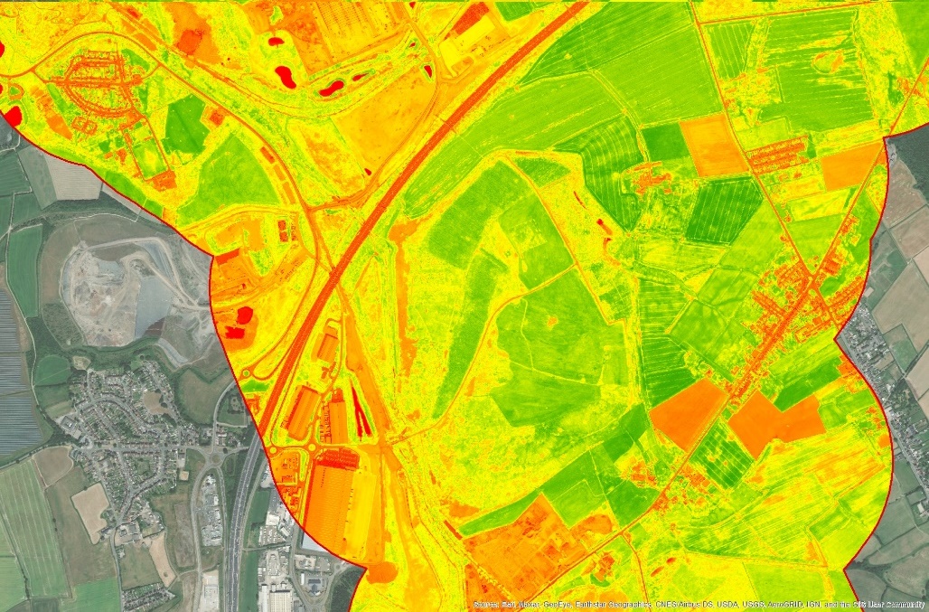
The spectral dataset used for this was NDVI, which is created using Equation (1).

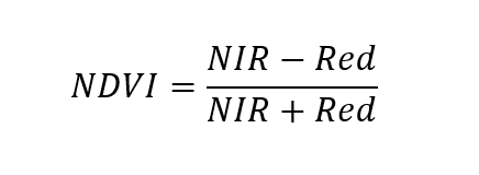
NDVI data (Figure 5) is an extremely effective tool for allocating general habitat types to different areas due to NDVI being a measure of surface reflectance, which provides a quantitative estimation of vegetation growth and biomass. The scale for NDVI is -1 to 1.

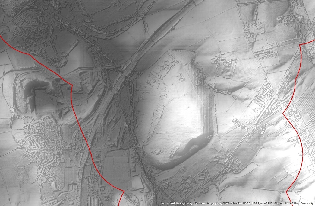
Other datasets used for the analysis included LiDAR DTM and DSM (Figure 6) to calculate the physical aspects of the habitats and NTM (Figure 7) created by BlueSky International.

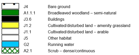
Classifications

Figure 8 shows the habitat classifications are determined using this methodology. The spectral and physical characteristics of these classifications have been derived from data accumulated from running the pre-classification method on other project sites as well as multiple small test areas within the HS2 site. HS2 survey data was then used to further refine the classicisation parameters.

Methodology

A pre-classification technique was created, tested, deployed using a semi-automated methodology that is outlined below. The output of this was a Phase 1 habitat pre-classification of HS2 Phase 2b.

The process of generating a pre-classified product started with creating a Digital Height Model (DHM), which along with spectral characteristics of the data is used to determine areas of potential scrub in the output pre-classification. DHM is created by taking the DTM and DSM LiDAR data, subtracting the DTM from the DSM, which is in effect removing the terrain of the earth’s surface and just leaving the elements on top such as vegetation and buildings. This dataset is then used to bring out the data which is of low height. Focal Statistics tool then determined areas with the largest variations in height, which effectively identifies areas of regular and irregular physical features. This data is then aggregated with the OSMM data and referenced to later determine potential habitat type.

The second stage is to take the NTM dataset and define areas of woodland and singular trees. This is done by looking at the whole data in relation to itself and determining where there are groups of trees with homogenous canopies where the expanse is greater than the JNCC Phase 1 Minimum Mappable Unit (MMU) of 0.1ha at a scale of 1:10,000. The trees that fall within this category are then dissolved together and lose their tree centre point to form a woodland polygon, whereas the trees that fall outside these parameters are just taken through as point data i.e. individual trees. This data is again aggregated to the OSMM data and referenced as per the previous stage (Figure 9).

At this stage the mean, max and minimum NDVI values are embedded into each OSMM polygon and this is used as the primary source of data for the characterisation of habitat of individual polygons. Multi-criteria analysis is used to determine the habitat type of each polygon by using multiple fields already in the OSMM GIS data along with the additional attributes added from the automated workflow.  Where the OSMM defines an area as manmade and the NDVI values confirm this (which we have found to be less than 0.05 spectral value) then that habitat type is defined as Hardstanding. A similar process is then undertaken to determine areas of water and buildings which the OSMM derives highly accurately.

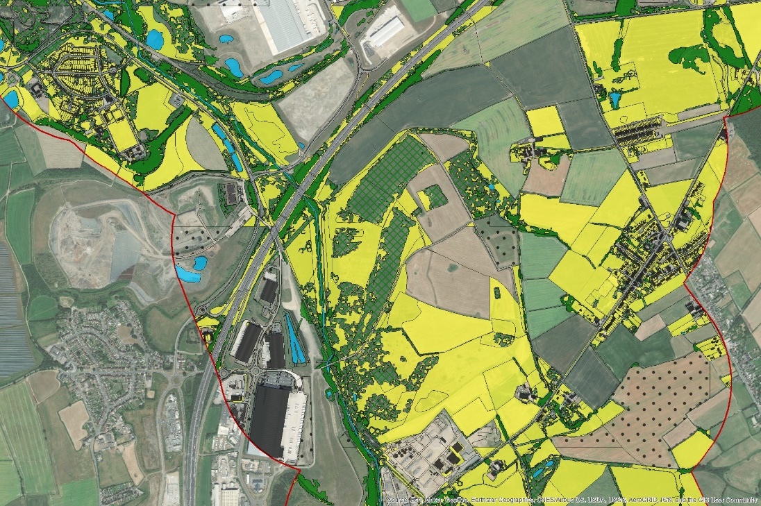
Each of the additional categories of habitat are then classified using all of the data within the OSMM to provide the most likely habitat classification for each polygon. For example, an area can have a scrub classifier but if the NDVI value suggests the vegetation reflectance is not intense enough, this is then reverted to OSMM descriptions of habitat. These final classified habitats (Figure 10) then go through an automated workflow to assign the JNCC codes and descriptions to them.

At the final step, the dataset is quality assured to find any systematic errors which are then corrected. The data is then uploaded to ArcGIS Online and made available to ecologists through ArcGIS Collector (a mobile data collection application) for verification through field surveys, which were undertaken using digital data capture methods.

Health and Safety

All HS2 Phase 1 surveys are carried out by experienced, specialist ecologists, working under formal safe operating procedures, as well as institutional best-practice. Surveyor safety is multi-faceted and can be influenced by a range of factors. Owing to the large scale and extent of surveys, the complexity of land access arrangements, topography, habitat types and accessibility across the survey areas, it is impossible to eliminate risks entirely. By providing the surveyor a pre-classified habitat map prior to survey, this facilitates better survey planning, adopting a targeted approach and reduces the burden on the surveyor to produce a geo-referenced habitat map whilst out in the field. The added confidence gained from extrapolated habitat data also reduces the need to access unsafe areas when ground-truthing and verification can be done in adjacent and similarly classified habitats. Overall, these factors cannot be discounted as significant safety benefits.

Accuracy and Coverage

The pre-classified map generated using the above methodology supports better accuracies with the possibility of covering larger areas. It has greater potential to overcome the challenges faced due to patchy access availability of a given site owing to land ownership permissions as well as Health and Safety restrictions as discussed above. These factors can otherwise have a significant impact on the inaccuracies and data gaps in habitat mapping. The promise of this method also lies in the potential for it to deliver information about key perspectives over large areas with regular temporal revisit periods, especially when considering the construction and post-construction monitoring requirements of HS2.

An MMU is defined as the smallest size entity to be mapped as a discrete feature. If large linear areas are mapped at spatial resolutions less than the effective MMU, this would not be repeatable and can cause significant difference in accuracy resulting in a ‘salt and pepper’ effect. This makes the choice of appropriate MMU clearly very important. The availability of very high-resolution satellite imagery (≤5m resolution) and on different temporal scales, has helped significantly to improve the MMU thus the appropriate confidence interval to support the accurate indentation and mapping of habitats over larger areas. The pre-classified map generated with the process presents much better confidence interval for the habitat maps compared to the aerial photographs even before getting into the field. Which is a further advantage as it can be doubly checked and verified easily when in field. In addition to this, the ground-truthing and extrapolation of the similar habitat type and condition will further increase the confidence levels supporting higher accuracy in habitat map production.

Another important factor while considering the accuracy of the generated habitat map is the inconsistencies which may creep in due to the different interpretation of methodology or habitat types by different surveyors of the large scheme of HS2. Subjective application of the observation of the extent, type and condition of habitat along with the variability in the extent of survey preparation add to it. Pre-classified product used in the process helped to overcome these challenges as it has significantly ruled out the possibilities of different interpretations by fixing it before going into the field. The OSMM along with the other datasets have helped to fix the habitat boundaries and variability of survey preparation to the greater extent. It has also helped the field surveyor to make the judicious use of the time by investing it into the complex habitat types rather than to larger homogenous patches. This way the suggested process flow has mitigated surveyor inconsistencies through controls includes standardising the starting point; eliminating subjectivity and human error by delineating habitats; standardising survey preparation through map production; facilitating better survey planning; and standardising map production to decrease variability in time spent in the field drawing. Also, the NDVI supported transitions between different habitat types or the condition of habitats even in homogenous areas, thereby increasing the accuracy by delineating them correctly and presenting them spatially to the surveyor to target field recording.

The accuracy of habitat accounting and duplication is another aspect that is significantly reduced when mapping is done manually. The feasibility and accuracy of this aspect is even more questionable when it needs to be used for larger areas such as HS2. Manual mapping undoubtedly creates slivers, gaps and overlapping polygons in the dataset which create difficulties with the accurate area calculation of habitats. Processing of data in GIS domain helps to overcome this problem by simply using clipping, snipping and editing functions for the shared boundaries with their topologies, providing a clean dataset from the outset. This provides a more accurate total polygon area, which supports early and effective decision making, particularly for the critical and important habitats where even the smallest difference in area can cause significant accounting/reporting errors in relation to mitigation and compensation planning. Pre-classified habitat map also helps increase the accuracies with the lower likelihood of errors creeping in through reduced processing and double handling of data by field surveyors and GIS specialists. The method means that the data is mostly handled by trained GIS specialists and verified by the field ecologists, which minimises the margin of errors which may otherwise result using a traditional workflow. The method also supports and strongly adds to QA procedures as it is more aligned with HS2’s progressive assurance approach. End-point QA typically forms part of the traditional Phase 1 workflow, however the Pre-classification method incorporates a QA process that is more progressive and continual, rather than allowing errors to creep into database at every stage risking final checks being done against the wrong dataset.

Efficiencies

Survey efficiencies realised from having pre-mapped habitat layers prior to site work starts with survey planning. Habitat maps during strategic survey planning stages informs decision making and forward planning of surveys. In the case of HS2, this output, in addition to other data including NDVI, NTM and biological records, allowed surveyors to effectively plan and target important areas for field survey and to ensure that field survey work was undertaken efficiently. This allows for more strategic planning to be undertaken, which may target more detailed information to be collected on a subset of habitats within a survey area. For example, where NDVI spectrums may highlight areas of potential conservation interest, thus allowing a targeted approach to be adopted.

On large linear infrastructure projects, it is appropriate to plan for efficient coverage of large areas of accessible land. The generation and provision of habitat maps prior to survey allows field surveyors to focus on recording data that traditional Phase 1 methodology does not translate easily into, including Priority Habitat Types or Habitats Directive Annex 1 types; information on condition, origin or management regime; and species lists^[23]. This is facilitated by surveyors not having to manually map spatial extents of habitats in the field. The time saving for ecologists in the field can also be realised where they have a digital device to collect the data and given that the geometries are already created, it turns manual mapping to an efficient process of simply changing the attribute data.

With a traditional survey methodology and workflow, the ecologist would be provided with paper maps and would then hand draw the information onto the map in the field. This would then be scanned in and send to the GIS analyst where they would have to geo-locate each image and then digitise that information. For large areas this would take significant time and would be subject to several revisions with high frequencies of errors due to the quality of scanned images. With the Pre-classification method used for HS2, all of the data was on an online portal where it could be downloaded and quality assured, this meant if there was a small geometry change required this could be done quickly and efficiently, with very little error created by the process itself. Whilst time-savings were not quantified for the HS2 Project, smaller urban case studies on projects across the UK had recorded GIS time savings being in the region of 40% with post-survey GIS time reduced in some cases by up to 90%.

Consultation

The methods set out in the SMR and FSMS follow recognised methodologies (deviating only where considered appropriate and with Natural England (NE) agreement) that have been determined in consultation with NE. NE are a recognised statutory consultee as part of the Environmental Impact Assessment process and whilst the pre-classification model did not technically present a deviation in the FSMS approach, it was recognised that NE should be engaged and consulted on the proposed approach. HS2 and MWJV met with NE on 12 October 2017 to discuss the method, context and application of the approach on HS2 Phase 2b. NE considered the method to be suitable for the requirements of the project and accepted that the approach had been designed to have a low computational impact. Further to this, consultation with JNCC, Adviser to Government on Nature Conservation, was undertaken on 8 October 2019 to discuss research and development opportunities and to learn more about Making Earth Observation Work[24] (MEOW), a four-phase project to address habitat monitoring and surveillance needs in the UK.

JNCC has developed the CRICK framework to support the monitoring & surveillance of the larger habitat areas and NE methodology take support of Earth Observation (EO) data to fill the field data gaps. On similar terms EAGLE group- The EIONET Action Group on Land Monitoring in Europe group have also created a framework that breaks Land Cover down into its constituent parts and a data model for analysing that basic data in different applications. Another example is Living Wales-which is an initiative of Welsh Government which works on basis of providing regular and consistent base variables that can be analysed depending on application.

In all the instances developed and used approaches are conceptually similar in terms of using Earth Observation and GIS data to support the larger area mapping and monitoring, but with the slight differences in approaches to achieve the respective goals. NE methodology is primarily to go out and undertake the survey in a traditional way wherever possible, and further use this data to define the parameters for each habitat type. This information is then extrapolated with the support of multi-spectral data to fill in the any gaps from the on-site survey. JNCC tends to use a machine learning method on multispectral satellite data to define the most likely habitat types. This is achieved from a training dataset for which the parameters are created from existing surveys. This is often used for very large areas on the dataset at 10-30m resolution. Similarly, the Pre-classification method also uses the rule-based approach to produce a habitat map prior to field work, but on the fixed major polygon boundaries taken with the OSMM and NDVI on a finer scale. The field work then further checks the doubtful/complex areas to ensure the habitat map accurately reflects the baseline condition and fulfils the project needs.

Applications and Development

A key element of remote sensing is to go out into the area covered by an image and make observations and measurements. This enables an effective extrapolation of verified information to produce an accurate product. High to very high resolution satellite data along with the pre-decided MMU can help to meaningfully extrapolate the ground observation and come up with a higher-accuracy Phase 1 habitat map, that could be developed further to incorporate land use, management, habitat condition and distinctiveness information for Net Positive analysis as well as Land and Asset assessments. Further information and field survey data that feeds into the current process will further allow the potential for machine learning to be incorporated such that the classification rules can be refined to reduce spectral mixing.

The Pre-classification method presents significant opportunities for long-term habitat monitoring, which can be effectively achieved because of the availability of a large amount of multi-temporal data from past and current spaceborne missions, with continuity provided by planned future missions. This approach means monitoring maps to identify change can be prepared and updated routinely.

Since 2015, the industry has recognised the disadvantages of the JNCC Phase 1 habitat classification system and a steering group was formed to develop a new system for classifying UK habitats^[23]. UK Habitat Classification (UKHab) has built on existing classification systems and integrates classification architecture that facilitates the recording of habitats at differing levels, from Broad habitat types, to Priority Habitats and Annex 1 habitats. The system also allows for direct translations from the existing classifications such as National Vegetation Classification (NVC)^[21] and Phase 1^[3], but also includes primary and secondary coding to allow the recording of habitat mosaics and management. Further development of the pre-classification system is required to catalogue and refine the rule-based system for interpreting UKHab classifications to enable a transition to the imminent replacement of the Phase 1 habitat classification. Further research should also look to incorporate hyperspectral data, currently used to support the remote identification of specific species^[25],[26].

Acknowledgements

We thank David Prys-Jones and Andrew Muir at HS2 Ltd who have provided guidance, review and proofing; Cristina Morrison at WSP who has provided graphic design input; and Natural England and JNCC for their time, discussion and insight relating to this work. The study was supported by HS2 Ltd, WSP and MWJV.

References

[1] CIEEM (2018). Guidelines for Ecological Impact Assessment in the UK and Ireland: Terrestrial, Freshwater, Coastal and Marine version 1.1. Chartered Institute of Ecology and Environmental Management, Winchester.

[2] CIEEM (2017). Guidelines for Preliminary Ecological Appraisal, 2nd edition. Chartered Institute of Ecology and Environmental Management, Winchester.

[3] JNCC, (2010). Handbook for Phase 1 habitat survey – a technique for environmental audit, JNCC, Peterborough, ISBN 0 86139 636 7.

[4] HS2 (2018). HS2 Phase 2b: Crewe to Manchester and West Midlands to Leeds Environmental Impact Assessment Report Scope and Methodology Report.

[5] HS2 (2017). HS2 Phase 2b: Technical note – Ecology and biodiversity – Ecological field survey methods and standards Document no.: 2EV01-ARP-EV-NOT-000-000064

[6] CIEEM (2017). Guide to Ecological Surveys and Their Purpose. Chartered Institute of Ecology and Environmental Management, Winchester.

[7] Burrough, P.A. and McDonnell, R.A. (1998). Principles of Geographical Information Systems. Oxford University Press, New York.

[8] Smith, G. F., O’Donoghue, P., O’Hora, K. and Delayney, E. (2011). Best Practice Guidance for Habitat Survey and Mapping. The Heritage Council.

[9] Cherrill, A.J. and McClean, C. (1999). Between-observer variation in the application of a standard method of habitat mapping by environmental consultants in the UK. Journal of Applied Ecology, 36: 989-1008.

[10] Laperriere, A. J., P. C. Lent, W. C. Gassaway, and F. A. Nodler (1980). Use of LANDSAT data for moose habitat analyses in Alaska, Journal Wildlife Management, 44:881-887.

[11] Dixon, R., B. Knudsen, and L. M. Bowles (1982). A pilot study of the application of LANDSAT data in the mapping of White-tailed Deer habitat in Manitoba. Land/Wildlife Integration No. 2 (H. A. Stelfox, and G. R. Ironside, editors). Lands Directorate, Environment Canada, pp. 91-95.

[12] Harris. R. (1983). Remote sensing support for the Omani White Oryx Project. Remote Sensing for Rangeland Monitoring md Management. Proceedings of the Ni Annual Conference of the Re- mote Sensing Society, Silsoe College, Bedford, pp. 17-2.

[13] Bowles, L. M. (1985). Integrated automated LANDSAT mapping into a large scale moose census program in northern Manitoba. Land1 Wildllife Integration No. 3 (H. A. Stelfox and G. R. Ironside, editors]. Ecological Land Classification Series No. 22. Land Conservation Branch, Environment Canada, pp. 99-104.

[14] Ormsby, J. P., and R. S. Lunetta (1987). Whitetail deer food availability maps from Thematic Mapper data, Photogrammetric Engineering 8 Remote Sensing, 53(8):1081-1085.

[15] Tornmewik, H., and I. Lauknes (1988). Inventory of reindeer winter pastures by use of LANDSAT-5 TM data, Proceedings of the International Geoscience and Remote Sensing Symposium 1988, Edinburgh, Scotland, p. 1223.

[16] Belward, A. S., J. C. Taylor, M. J. Stuttard, E. Bignal, J. Matthews, and D. Curtis, (1990). An unsupervised approach to the classification of semi-natural vegetation from Landsat Thematic Mapper data. A pilot study on Islay. International Journal of Remote sensing, 11:429-445.

[17] Fuller, R.M., Cox, R., Clarke, R.T., Rothery, P., Hill, R.A., Smith, G.M., Thomson, A.G., Brown, N.J., Howard, D.C., Stott, A.P. (2005). The UK land cover map 2000: planning, construction and calibration of a remote sensing, user-orientated map of broad habitats. International Journal of Applied Earth Observation and Geoinformation 7 (3), 202–216.

[18] Fuller, R.M., Groom, G.B., Jones, A.R. (1994). The land-cover map of Great Britain: an automated classification of landsat thematic mapper data. Photogrammetric Engineering and Remote Sensing 60 (5), 553–562.

[19] Fuller, R.M., Smith, G.M., Sanderson, J.M., Hill, R.A., Thomson, A.G. (2002). The UK land cover map 2000: construction of a parcel-based vector map from satellite images. Cartographic Journal 39 (1), 15–25.

[20] Lucas, R.M., Rowlands, A., Keyworth, S., Brown, A., Bunting, P. (2007). Mapping habitats and agricultural land covers in Wales using multi-temporal remote sensing data. ISPRS Journal of Photogrammetry and Remote Sensing 62 (3), 165–185.

[21] Rodwell, J.S. (2006) NVC Users’ Handbook, JNCC, Peterborough, ISBN 978 1 86107 574 1.

[22] Smith, G.M., Wyatt, B.K. (2007). Multi-scale survey by sample-based field methods and remote sensing: a comparison of UK experience with European environ- mental assessments. Landscape and Urban Planning 79 (2), 170–176.

[23] CIEEM (2018) Introducing the UK Habitat Classification – Updating Our Approach to Habitat Survey, Monitoring and Assessment. In Practice. Issue 100, Bulletin of the Chartered Institute of Ecology and Environmental Management

[24] Medcalf, K.A., Parker, J.A., Turton, N. & Bell, G. (2014). Making Earth Observation Work for UK Biodiversity – Phase 2. JNCC Report No. 495, Phase 2, JNCC, Peterborough, ISSN 0963-8091.

[25] Cushnahan, Tommy & Yule, Ian & Pullanagari, Rajasheker & Grafton, Miles. (2016). Identifying grass species using hyperspectral sensing.

[26] Bellanti, L., Blesius, L., Hinnes, E., & Kruse, B. (2016). Tree species classification using hyperspectral imagery: A comparison of two classifiers. Remote Sensing, 8(6), 445–463.